Research, Analysis, & Point of View

Key Takeaways

• Decarbonizing steel is key to meeting ambitious climate targets in the face of rapidly expanding AI infrastructure as well as broader infrastructure growth.
• The gap between corporate climate ambitions and near-term commercial reality is widening. Despite strong demand signals from hyperscalers and other major buyers, leading producers have recently canceled or delayed flagship green steel projects, citing high energy costs, slow hydrogen market development, and unfavorable policy environments. 
• Bridging this gap requires significant capital investment and supporting mechanisms to scale low-carbon technologies. Environmental attribute certificates offer an effective mechanism to channel capital toward transformative, low-carbon steel projects, supporting technology scale-up, as well as providing a way for buyers to meet their emissions reduction targets.  
• To protect the credibility of environmental attribute certificates as a market mechanism for decarbonization, projects should seek to meet rigorous quality criteria such as additionality, verifiability, and catalytic impact.

Forging New Climate Ambitions for Steel Production

Decarbonizing steel production is essential to meet global climate targets. Steel production accounts for approximately 7–9% of global CO₂ emissions. This is driven chiefly by coal-based primary steelmaking, which still accounts for the majority of global production. Globally, at least 1.8 billion tonnes of crude steel were produced in 2025 to serve a broad array of industries including real estate, infrastructure, automotive, and data center construction. 

As hyperscalers race to build the infrastructure underpinning the AI revolution, steel demand for data center construction, and associated energy infrastructure, is increasing. While the relative share of data center demand for steel versus global steel demand is small, the need for approximately 20,000 tonnes of steel per data center has a material impact on hyperscaler’s public climate commitments. Microsoft, Meta, and other large technology companies have set ambitious 2030 climate targets that include their scope 3 emissions. The embodied carbon of the steel used to build their data centers sits squarely in scope 3.

Hyperscaler’s climate commitments have generated sector-specific demand for decarbonized steel, presenting an opportunity to affect steel decarbonization more broadly. Despite this demand, the supply of low-carbon steel remains limited. The industry faces significant scale-up challenges due to the diffuse nature of demand and the nascent market. Catalyzing growth in decarbonized steel production will require market innovations and new production pathways designed to overcome these challenges. Credible environmental attribute certificates can help bridge the gap between today’s market and tomorrow’s low-carbon steel sector.

What is an Environmental Attribute Certificate?

An environmental attribute certificate (EAC) represents the environmental attributes of a product that can be unbundled and transacted separately from the underlying physical commodity. The most widely used EACs today are renewable energy certificates (RECs), which track the environmental attributes of renewable electricity. The same concept can also be applied to steel and iron, as well as to materials such as cement and concrete.

In a book and claim model, a steel producer can implement a verified emissions reduction intervention, quantify the resulting lowered carbon intensity per tonne of steel produced, and convert that into tradeable certificates. Buyers can then purchase those certificates to support the deployment of low-carbon steelmaking capacity in cases where direct procurement of low-carbon steel is currently impractical due to geographic, contracting, or scheduling incompatibilities.

EACs are distinct from carbon credits. They do not represent emissions reduced or avoided relative to a counterfactual; they represent the intrinsic carbon intensity of the material produced, measured through a life cycle assessment. 

Decarbonizing Steel Requires Significant Capital and Infrastructure Deployment

Steel Production Today

Steel is currently made via three main production routes. About 71% of the world’s steel is produced through the blast furnace–basic oxygen furnace (BF-BOF) route, which emits an average of 2.33 tonnes of carbon dioxide (tCO₂) per tonne of crude steel. A further 24% is produced using scrap-based electric arc furnaces (EAFs), which emit 0.68 tCO₂ per tonne on average—far lower, but still dependent on the carbon intensity of grid electricity. The remaining roughly 5% uses direct reduced iron combined with an EAF (DRI-EAF), typically using natural gas, emitting 1.37 tCO₂ per tonne on average.

While increasing scrap-based production is a critical decarbonization lever, scrap availability is limited. Primary steel production, which uses iron ore as the main feedstock rather than recycled scrap, will remain necessary at large volumes through 2050. This makes it essential to decarbonize ore-based pathways, especially ironmaking: the step where iron ore is reduced to iron and where most emissions occur.

Decarbonizing ore-based steel production requires one of three fundamental interventions: (1) replacing coal and natural gas with low-carbon fuels such as hydrogen or bio-coke, (2) electrifying ironmaking directly, or (3) capturing and storing the CO₂ generated from fossil-fuel-based processes. All three involve significant capital expenditure and dependencies on infrastructure that is not yet in place at the necessary scale. As a result, the energy and cost challenge is substantial.

Low-Carbon Steel: Emerging Pathways

A range of transformative technological pathways are currently in development to overcome these barriers, offering the potential to deliver deep decarbonization to the steel industry exceeding 90% by 2050: 

• Hydrogen-based DRI-EAF: Using green hydrogen instead of natural gas within the DRI process provides a pathway to significantly lower the carbon intensity of ironmaking. Producers such as Stegra are deploying commercial-scale facilities designed to utilize 100% green hydrogen to reduce iron ore.
• Electrifying ironmaking: 
  
  • Molten oxide electrolysis: Boston Metal is commercializing a process that uses electricity to directly convert iron ore to molten metal through electrolysis at high temperature, eliminating the need for hydrogen or carbon reductants entirely.
  • Low-temperature electrowinning: Colorado-based startup Electra uses renewable electricity to extract iron from ore via an aqueous electrochemical process that operates at near-ambient temperature. 
• Carbon capture and storage (CCS): For blast furnaces and DRI plants with long remaining lifetimes, retrofitting with CCS technology can significantly reduce emissions. With new high-emitting capacity still being built, and assets expected to operate for decades, integrating CCS will be essential to avoid long-term carbon lock-in and to decarbonize these facilities over time. To date, commercial-scale deployment remains limited. The Al Reyadah facility at Emirates Steel is the only project currently capturing CO₂ from a DRI process at scale, though a handful of other large-scale projects have entered the development pipeline.

Progress and Setbacks: A Mixed Picture

The past year sent contradictory signals about the pace of steel decarbonization. On the demand side, technology companies with ambitious climate targets are actively signaling their intent to procure near-zero steel and support its development.

In September 2025, Microsoft and Stegra announced a landmark agreement that combines a physical supply deal for low-carbon steel with a separate EAC purchase agreement. Around the same time, Meta announced an agreement with Electra to purchase EACs tied to the startup’s clean iron production, becoming one of the first buyers to use the EAC model for an entirely novel, pre-commercial ironmaking technology. Nucor, the largest US steelmaker, also entered into a physical iron purchase agreement with Electra.

Despite these demand signals, the industry has experienced significant setbacks. A series of low-carbon steel project cancellations and delays has raised questions about the pace and viability of the steel transition, especially due to the high costs associated with green hydrogen production.

At present, the green premium for most low-carbon steel remains too high for buyers. A combination of sustained policy support, long-term demand signals from buyers willing to pay more, and scaling of supporting industries, such as green hydrogen production, is necessary for the low-carbon steel industry to be successful in the long run.

How EACs Can Bridge the Funding Gap in Steel

EACs unbundle low-carbon steel attributes from the physical material, reducing the friction between buyers who are willing to pay a green premium and geographic or logistical constraints that may inhibit physical offtake. Buyers, such as hyperscalers procuring conventional steel for data center construction in locations where low-carbon steel is not yet available, can purchase these certificates to support the development of low-carbon capacity, attribute lower-carbon production to their steel use via a market-based mechanism, and advance toward their scope 3 targets.

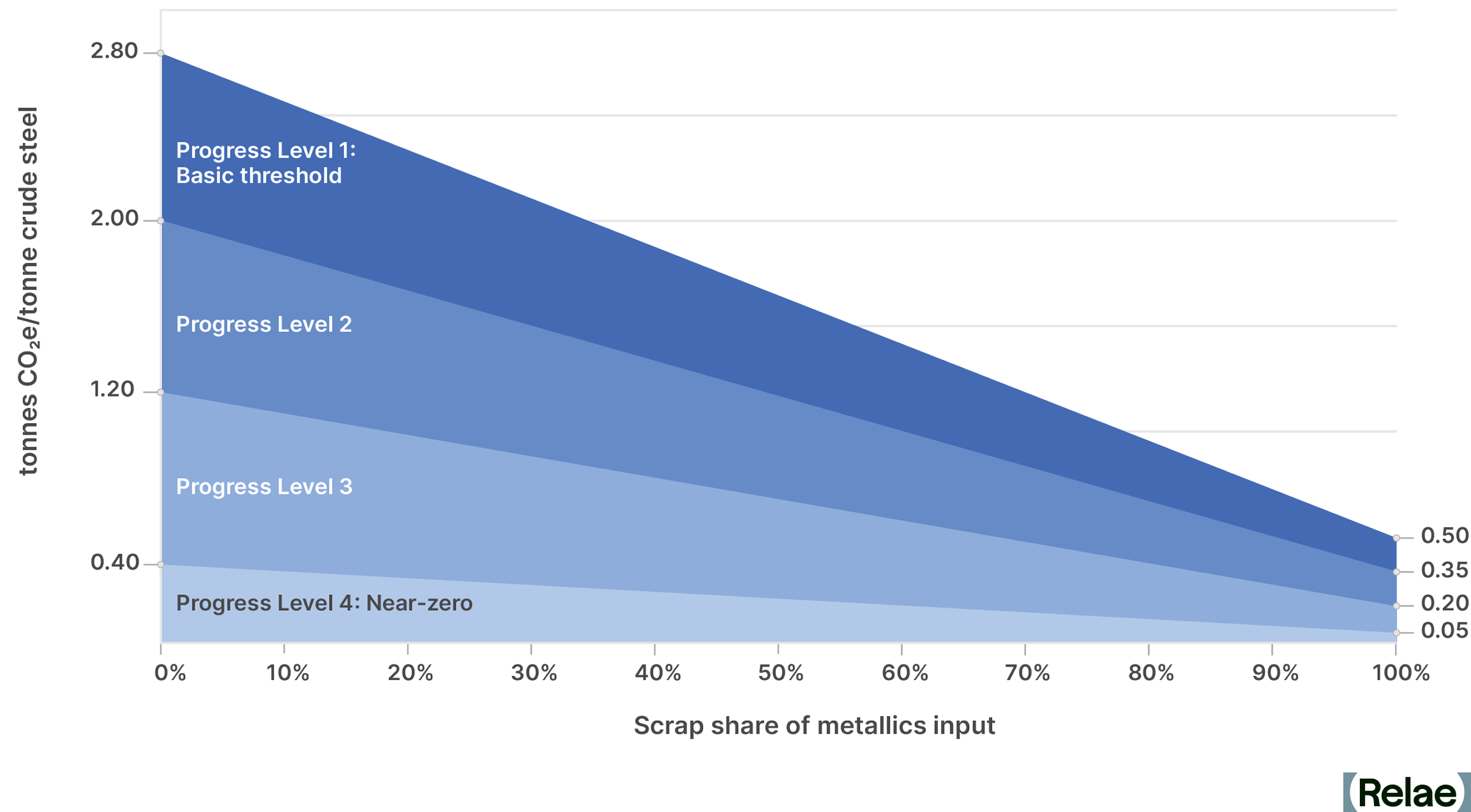
A primary objective of the Criteria for High-Quality Environmental Attribute Certificates in the Concrete and Steel Sectors, jointly developed by Relae (formerly Carbon Direct) and Microsoft, is to establish high-integrity standards for the EAC market in these sectors. For steel EACs, that means demonstrating significant emissions reduction performance by reaching at least Progress Level 2 in the ResponsibleSteel Decarbonization Progress Levels framework, and aiming to achieve Progress Level 3 by 2030. ResponsibleSteel’s scrap-variable benchmark provides a technology-neutral mechanism to evaluate emissions reduction performance by accounting for the specific proportion of scrap used.

EACs for steel are designed to be catalytic. Rather than supporting incremental improvements that are already becoming cost-competitive, they should target transformative capital changes, such as replacing BF-BOF routes with DRI-EAF, adopting low-carbon hydrogen in DRI processes, or deploying novel ironmaking technologies. Multi-year purchase agreements are particularly powerful because they provide the investment certainty that first-of-a-kind projects need to access capital at a lower cost.

What this Means for Buyers and Suppliers of Low-Carbon Steel 

Whether you are producing or procuring steel, EACs are only one part of a broader decarbonization strategy. For buyers with significant emissions from steel, and other building materials such as cement and concrete, EACs can be a powerful tool to help advance scope 3 reduction goals where supply for physical low-carbon materials is limited. Suppliers can complement commercialization strategies for low-carbon materials by using EACs to monetize emissions reductions, generate additional revenue to support decarbonization investments, and help scale markets for low-carbon materials. Navigating the steel market requires decisions at the intersection of technical feasibility, greenhouse gas accounting, and capital strategy. Key considerations include:

• Greenhouse gas accounting and reportability: Cradle-to-gate emissions for steel production must be tracked using life cycle assessments and should strive for interoperability with environmental product declarations (EPDs). EAC transactions must be reported transparently, especially given the absence of formal market standards at this stage.
• Additionality and catalytic impact: EAC purchases must demonstrably support projects that would not proceed without financial support from the EAC market mechanism, and projects should have a credible pathway toward the near-zero (Progress Level 4) threshold on the ResponsibleSteel framework.
• Avoiding double counting: EAC buyers must verify that the environmental attributes they purchase are not also being claimed by the physical product buyer via an EPD.

FAQs

What is an environmental attribute certificate (EAC) for steel?
An EAC represents the environmental attributes of low-carbon steel, unbundled from the physical material itself, so a producer can quantify a verified reduction in carbon intensity per tonne and sell that value as a separate, tradeable certificate. Buyers can purchase EACs to support low-carbon steel production while still working toward their own emissions targets.

How is an EAC different from a carbon credit?
An EAC reflects the intrinsic carbon intensity of the material itself, measured through a life cycle assessment. That's different from a carbon credit, which represents carbon dioxide actively avoided, reduced or removed from the atmosphere relative to a baseline.

How are AI data centers impacting the demand for low-carbon steel?

Data centers use roughly 20,000 tonnes of steel each, and as hyperscalers build out AI infrastructure, that steel use counts toward their scope 3 emissions and public climate targets. That's turned data center construction into a meaningful driver of demand for low-carbon steel, even though supply remains limited.

What makes an EAC credible enough to count toward a company's emissions goals?
A credible steel EAC needs to meet criteria like additionality (the project wouldn't happen without the EAC revenue), verifiability through life cycle assessment, and catalytic impact toward transformative technology rather than incremental gains. Relae (formerly Carbon Direct) and Microsoft jointly developed criteria for high-quality EACs in the steel and concrete sectors, which set a threshold of at least Progress Level 2 on the ResponsibleSteel Decarbonization framework today, rising to Progress Level 3 by 2030.

Can a producer sell an EAC and also get credit for the physical steel elsewhere?
No. EAC producers need to confirm the environmental attributes they're selling aren't also being claimed by whoever buys the physical steel through an environmental product declaration; otherwise the same emissions reduction gets counted twice.

Key Takeaways

• CORSIA, the program intended to address international aviation emissions, is currently the world’s largest international compliance carbon market, with approximately 200 million tonnes of eligible emissions units (EEUs) expected to be retired for Phase 1 (2024-2026) compliance. 
• Airlines have already begun retiring significant volumes of credits (clean cookstoves and jurisdictional REDD+) toward their Phase 1 obligations ahead of the January 2028 compliance deadline, signaling that the industry is treating CORSIA as a binding policy mandate.
• In addition to the four already approved, a record 25 carbon standards have applied for eligibility to supply credits under Phase 2 (2027–2035), pointing to a diversifying pipeline of credits.
• Legal enforcement of CORSIA at the national level remains uneven. A handful of jurisdictions, including the EU, Japan, Brazil, New Zealand, and Canada, have established compliance regimes, but it is unclear whether other major aviation markets will implement domestic enforcement requirements by 2027.
• As CORSIA matures alongside other compliance and voluntary frameworks, strategic engagement increasingly depends on understanding where eligibility overlaps and where the most value can be found.

Introduction to CORSIA 

The Carbon Offsetting and Reduction Scheme for International Aviation (CORSIA) was established and is managed by the International Civil Aviation Organization (ICAO)—a specialized agency of the UN—and provides a compliance mechanism to reduce emissions from international aviation that do not fall within a single country’s contributions to the Paris Agreement. For years, CORSIA generated more commentary than activity—airlines weren’t required to offset a single tonne of CO₂ emissions (tCO₂) during the pilot phase (2021–2023). That is changing; in early 2026, Singapore Airlines and Japan Airlines retired significant volumes of carbon credits against their Phase 1 (2024–2026) obligations. Increasing authorization announcements showcase the eligible supply steadily entering the market, and 25 carbon standards have applied for Phase 2 (2027–2035) eligibility. As CORSIA becomes an active compliance market, this article explains how the program works, what is driving the current trends, and what to watch as Phase 1 draws to a close.

Who is Covered by CORSIA Phase 1 and Phase 2?

Because emissions from international aviation are not tied to any individual nation, the International Civil Aviation Organization (ICAO) adopted CORSIA in 2016 to complement the Paris Agreement framework and address these emissions. CORSIA applies to international airlines operating flights registered between participating countries. 

• During Phase 1, offsetting obligations apply only to routes between the 130 countries that have voluntarily opted in. 
• From Phase 2, participation becomes mandatory for all 193 ICAO member states, except for those below the aviation activity threshold or classified as Least Developed Countries, Small Island Developing States,  or Landlocked Developing Countries—although they can voluntarily participate. 

Several major aviation markets, including China, that are not participating in Phase 1 will be required to do so from 2027. 

Offsetting Obligations

Airlines are required to offset the portion of their emissions that exceeds the program’s baseline on routes subject to offsetting. The key input is the annual Sectoral Growth Factor (SGF), which reflects how much annual emissions on covered routes have grown above the baseline (set at 85% of 2019 emissions). In simple terms, each airline's offsetting obligation is calculated by multiplying its CORSIA-regulated emissions by the SGF.

For example, an airline that emits 1 million tCO₂ on covered routes in a year when the SGF is 10%, would have an offsetting obligation of 100,000 tCO₂. An airline that emits 500,000 tCO₂ in the same year would have an obligation of 50,000 tCO₂. The actual 2024 SGF was 15.4%, exceeding the baseline and triggering offsetting obligations for the first time since the COVID-induced reduction in international aviation activity. 

Beginning in 2033, CORSIA’s offsetting formula combined the SGF with an individual component that accounts for each airline's own emissions growth. The individual weighting starts at 15% in 2033 (with an SGF weighting of 85%) and rises to 45% by 2035 (SGF 55%). This progressively ties each airline’s obligations to its own emissions trajectory rather than sector-wide trends alone.

Airlines can also reduce their obligations by reporting the use of CORSIA Eligible Fuel (CEF). In order to qualify as CEF, Sustainable Aviation Fuel (SAF) must meet ICAO’s certification criteria. Offsetting remains a lower-cost option than sustainable fuel procurement, and CORSIA obligations are currently not influential drivers of CEF/SAF uptake compared to supply mandates, such as ReFuelEU Aviation. However, these dynamics will evolve as CORSIA matures and SAF prices continue to fall. 

CORSIA Eligible Carbon Credits: Phase 1 and Phase 2 

To determine the eligibility of carbon crediting standards and credits issued under those standards, ICAO's Technical Advisory Body (TAB) reviews applications and recommends approval to the ICAO Council, subject to restrictions on methodologies, vintages, and more granular project elements. Currently, no standard is approved without exclusions. Credits eligible for use under CORSIA are known as Eligible Emissions Units (EEUs).

‍

‍

TAB broadly excludes some project types across standards, including large-scale grid-connected renewable energy projects and most project-level REDD+ activities. The exclusions reflect TAB's assessments of baselines, safeguards, and quantification gaps. However, these assessments are not static; ICAO updates its determinations as the evidence base improves. For example, in 2025, TAB approved certain direct air capture (DAC) and biochar pathways for the first time.

A record 25 carbon standards—certifying projects from emissions avoidance to engineered carbon dioxide removal (CDR)—have applied for Phase 2 eligibility in the 2026 assessment cycle, reflecting the scale of the opportunity. The International Air Transportation Association (IATA) projected a demand of 170–236 million EEUs for Phase 1 alone; developers are eager to serve this growing market. Assessment results are expected in October 2026.

Article 6 and Corresponding Adjustments

The biggest bottleneck for eligible supply has been requirements relating to Article 6.2 of the Paris Agreement. CORSIA requires that EEUs carry a host country Letter of Authorization (LoA) confirming that the host country will not count the underlying mitigation toward its Nationally Determined Contribution (NDC). This prevents double counting between CORSIA and national emission inventories, but it also means eligible supply depends on host country authorization, not just meeting methodological requirements. Authorized credits are called Internationally Transferred Mitigation Outcomes (ITMOs). 

To manage the risk that a host country fails to apply the promised corresponding adjustment, projects must secure legally enforceable insurance policies that either provide replacement EEUs or funds to secure them. Several providers have been approved to insure EEUs registered by Gold Standard and Verra. 

Insurance requirements do not apply when the host country has already confirmed the corresponding adjustments in its mandatory Paris Agreement reporting. For example, in March 2026, Madagascar submitted a Biennial Transparency Report (BTR) and annual information report that reflect the application of corresponding adjustments to CORSIA-eligible clean cookstoves credits listed on the Verra registry. According to Verra, BTR accounting is the “highest level of assurance” that ITMOs will not be double counted. 

The Enforcement Challenge

With the authorization bottleneck loosening, market attention is turning to demand. Critically, ICAO has no direct enforcement power; for CORSIA to work, participating countries must pass laws requiring airlines to comply with its requirements. Under CORSIA rules, airlines must retire their Phase 1 EEUs by January 2028, but most are not yet subject to legal sanctions for failing to comply. Where regulations do exist, it remains unclear whether penalties will be stringent enough to matter, or whether they will be enforced at all.

Where legal enforcement of offsetting requirements does exist, it varies by design. For example, in Brazil, failure to comply attracts a penalty of BRL 50/tCO₂ (US$10/tCO₂) and an administrative fine. Meanwhile, the Canadian Aviation Regulations impose administrative fines capped at CAD 25,000 (US$18,000) per infraction, but there is no specific fine for each tCO₂ not offset. However, the absence of a statutory penalty framework does not necessarily mean compliance will not be enforced. For example, New Zealand manages CORSIA participation through an administrative Memorandum of Understanding with Air New Zealand, rather than a dedicated legal regime (though this will change from 2027). Similar informal arrangements may be more common than the legislative record suggests.

According to 2024 data, US-based airlines account for around 15% of CORSIA-covered emissions. However, there is no indication that the federal government will implement CORSIA penalties under the current administration. It is unclear how non-compliance by a major economy will impact market confidence or enforcement by other governments, but uncertainty about US participation in multilateral climate programs is not new. 

What to Watch

• Global enforcement: As Phase 2 approaches, the prospects for CORSIA enforcement in key aviation markets will become clearer. China, which has not participated in the voluntary phase and has raised objections to CORSIA’s design on grounds of fairness, presents an uncertain picture for domestic transposition. The UK government has consulted on a draft legal amendment that would penalise non-compliance for UK airlines at £100/tCO₂ (US$130/tCO₂), but has not published updates since February 2025. 

• EU Emissions Trading Scheme (ETS) update: In July 2026, the European Commission proposed to expand the ETS to address emissions from flights departing the European Economic Area (EEA) to destinations within 5,000 km. To avoid double charging emissions also regulated under CORSIA, the Commission proposed to deduct CORSIA costs from airlines’ ETS obligations. While the Commission flagged concern about the stringency of CORSIA eligibility criteria, the proposed rules would not impact demand for Phase 1 EEUs. Still, it is worth watching for future restrictions on which credits EU airlines can use for CORSIA, whether in Phase 1 or 2. 

• Supply financing vehicles: The LEAF Coalition—which purchases credits verified under the CORSIA-eligible ART TREES standard—has signed over US$1.5 billion worth of purchase agreements with host countries. The Forest Carbon Partnership Facility (FCPF) and BioCarbon Fund Initiative for Sustainable Forest Landscapes (ISFL), both CORSIA-approved for Phase 1 in early 2026, have built jurisdictional REDD+ pipelines across dozens of countries. As projects mature, it will be worth watching how issued credits are marketed across compliance and voluntary channels.

Strategic Considerations

Avoided emissions credits dominate early CORSIA supply—and consequently demand—principally from avoided deforestation and clean cooking projects. As there is no regulatory premium for higher-cost CDR, this is not surprising. But as the market matures and supply diversifies, airlines are likely to begin differentiating on geography, co-benefits, and environmental performance. Corporate interest is growing in projects that abate non-CO₂ superpollutants, due to their outsized near-term climate impact. As many of these projects are based in countries actively issuing LoAs, this may soon translate into a supply of superpollutant EEUs. Some airlines are reluctant to procure aggressively now, anticipating the upcoming availability of higher-quality credits.

Credits that hold value across multiple frameworks could carry a strategic premium. A credit also eligible for Singapore's carbon tax, Switzerland's CO₂ Act, or SBTi claims may offer more durable demand than one tied to a single use case. While specific requirements vary significantly, we are beginning to see convergence around broad principles, such as the need for Article 6 authorization for credits used in compliance markets tied to NDCs. Procurement and project development strategies could begin to favour credits that confer wider market optionality. 

The precondition for all of this is policy stability. Longer-term offtake agreements, portfolio strategies, and meaningful investment in project development depend on confidence that CORSIA rules will hold. Efforts to soften emissions regulations in response to energy price shocks are now testing this confidence, from proposed changes to soften the EU ETS to Singapore's deferral of its SAF levy. Tracking price signals, enforcement developments, and authorization trends will be essential for identifying firm demand and where the opportunities lie.

Conclusion

Effective engagement with CORSIA requires more than developing quality projects. It means understanding methodological eligibility requirements, navigating Article 6.2 authorization processes, tracking a network of overlapping national regulations, and staying ahead of a rapidly evolving market landscape. Relae (formerly Carbon Direct) brings together policy, market, and scientific expertise to help clients on all of these fronts.

Frequently Asked Questions

Which carbon credits can airlines use for CORSIA compliance?

CORSIA Eligible Emissions Units (EEUs) must be issued by crediting standards approved by ICAO's Technical Advisory Body. Every approved standard currently has exclusions on certain methodologies and project types, so eligibility is granular rather than blanket. EEUs must also have a host country Letter of Authorization confirming a corresponding adjustment under Article 6.2 of the Paris Agreement.

Is CORSIA actually enforceable?

In all phases, CORSIA obligations are legally binding when a country writes them into domestic law. Countries participating in Phase 1 are expected to do this, but not all have, and enforcement remains uncertain in several key aviation markets (e.g., the United States). Even where enforcement exists, penalty regimes vary significantly in stringency and design. 

How does the July 2026 EU ETS proposal affect CORSIA?

The European Commission's proposal to expand ETS coverage to more flights does not reduce demand for CORSIA credits. While it would lead to overlap between flights covered under CORSIA and the ETS, as proposed, airlines could have CORSIA costs effectively deducted from their ETS allowance obligations. However, the Commission has signalled continued scrutiny of CORSIA's effectiveness, which could shape future limits on the credits EU airlines are allowed to use.

Key Takeaways

• Agentic inference has changed the economics of AI. Tokens are becoming units of work and the economic driver is now the work produced, not token generation. Per-token costs are falling and the willingness to pay for work produced is rising; these two trends compound. This tailwind enhances AI economics and has spillover impacts on all layers of the AI stack.
• The AI infrastructure question has shifted from whether demand will show up to whether the physical stack can scale quickly enough. That stack includes power generation, grid capacity, interconnection, compute, memory, networking, cooling, siting, and community acceptance.
• Carbon Direct Capital and Relae (formerly Carbon Direct Inc.) have a differentiated view because the two entities work across both sides of the constraint: Relae advises hyperscalers and energy buyers on power and grid bottlenecks, while Carbon Direct Capital invests in the technologies that relieve those bottlenecks.
• Carbon Direct Capital sees better risk-adjusted returns investing in the physical foundations of AI, including clean firm power, energy system efficiency, data center efficiency, and inference-optimized compute, rather than chasing late-stage AI application valuations.

A Better Question Than "Is AI a Bubble?"

The most important development in AI economics is agentic AI turning tokens into work, a shift that reframes the bubble debate which dominated investor conversations, sell-side notes, and Chief Information Officer surveys through early 2026. Hyperscalers spent approximately US$380 billion on capital expenditure (capex) in 2025 and have guided to approximately US$720 billion of capex in 2026.¹ Carbon Direct Capital and Relae have worked together to build project-level models for both training and inference facilities to demystify the numbers and understand financial and technical sensitivities. The core finding was that the assets could be bankable using standard assumptions and that the binding constraints were physical, not financial. That conclusion has been reinforced in recent months by new developments.

Concretely, AI is moving from single prompts and answers to multi-step workflows that plan, reason, call tools, verify outputs, and keep state. This shift to inference is the structural successor to training in the initial AI capex cycle; it changes power requirements, time to power, and compute architectures all at once. Goldman Sachs estimates that agentic AI could drive a 24-fold increase, relative to a 2026 baseline, to roughly 120 quadrillion tokens per month globally by 2030 as per-token costs continue to fall. SemiAnalysis makes the same point from another angle: the value of frontier tokens has risen as agentic workflows become useful, while hardware and software improvements have reduced the cost of producing each token.

This does not mean every AI company is attractive, every data center project works, or every valuation is justified. It means the easy bubble framing is missing the more investable question. If token demand is compounding and the unit value of work produced is rising, the scarce resource is not abstract enthusiasm. It is the physical infrastructure required to turn that demand into work produced.

The Data Center Model Still Matters, But the Box is not a Black Box

Our internal modeling for an illustrative 167-megawatt inference data center using Nvidia Blackwell graphics processing unit (GPU) servers suggests the potential for high-teens percent equity returns under a defined set of assumptions.² We built a bottom-up underwriting, beginning with the number of users served per inference data center, assuming approximately how many tokens they will demand daily, and translating that token demand into compute needed based on industry-standard quantization and utilization rates. We then inferred the number of GPUs and servers needed to achieve the desired compute, which ultimately drove the total invested capital and power demand based on assumed thermal power designs and power usage effectiveness (PUE). On the revenue side, we used GPU-as-a-service rental rates as one proxy for the market value of compute capacity. A hyperscaler would not rent scarce compute externally if it had higher-value internal demand for that same capacity. As we will detail below, GPU rental prices have been steadily increasing on the back of inflecting inference demand.

This model is not the entire argument; it is the starting point. An important lesson is that power cost alone does not break data center economics. Electricity is slightly over 10% of total costs in our model: a 50% increase in power price reduces equity-level returns by less than 2%. Access to power, speed of interconnection, and equipment availability matter more. In other words, the economics of the model facility are workable, but only if the facility can be built and powered on the timeline customers need.

That is where most AI commentary remains too superficial. It treats the data center as a black box: capex goes in, tokens come out. That misses the bottlenecks inside and around the box. AI racks are moving far beyond traditional cloud power density. Cooling is shifting from air to liquid and two-phase systems. Networking and high-bandwidth memory become binding constraints in inference architectures. Grid interconnection queue wait times stretch to years. Communities can and do block projects. The technical, physical, and political constraints are increasingly the drivers of potential returns.

Inference Makes the Constraint Structural

While training is episodic, inference is recurring. A training run can be delayed, accelerated, or redesigned. Inference happens every time a user asks a question, a developer runs an agent, a business automates a workflow, or an application calls a model in the background. Agentic inference multiplies that load because one user action can become many model calls, validation loops, and memory reads; industry benchmarks show that agentic systems consume 5–30 times more tokens than a standard chat interaction.

Inference demand is also resilient in both directions. If efficiency gains lower the cost per token, more workflows become economic and total token consumption rises - the classic Jevons Paradox. However, token prices do not necessarily need to fall for inference spend to grow. As the economic unit shifts from tokens generated to work produced, customers may pay more per token when an agent delivers work produced that is worth more than the inference cost. Regardless of token price, tokens must all route through the same physical bottlenecks and we are seeing an increase in inference demand.

The architecture of inference is also changing. Some workloads will prioritize low-latency answers. Others, especially agentic work without a human waiting on every token, will prioritize memory, state, context, and cost per completed task. That means the AI infrastructure stack will become more heterogeneous, not less: XPUs (specialized AI accelerator chips), custom silicon, photonics, memory hierarchies, and edge or regional deployment models will all matter. The pricing data shows demand for more AI infrastructure overall: on-demand GPU rental capacity is effectively sold out across all chip generations in early 2026, with one-year Hopper H100 contract pricing rising 15–20% month-on-month through March 2026 and Blackwell B200 rental rates up 23% in March alone. When rental rates rise into a wave of new chip supply, supply is not catching up to demand.

Power Is Not One Constraint, It Is Several

Saying "AI is power constrained" is true, but not specific enough. The real problem has several layers. First, data centers need more electricity than many local grids can deliver on hyperscalers' timelines. Crucially, some grids can supply sufficient power but not continuously for 8,760 hours per year, conflicting with traditional assumptions about service reliability and leading to novel strategies around flexibility and intermittent self-supply. Second, the grid must be able to absorb large, fast-moving computational loads without creating reliability risks. Third, customers need energy procurement strategies that satisfy cost, reliability, climate, and public-acceptance requirements. Fourth, projects must get built in real communities, through real interconnection processes and real permitting fights. Power is not simply a commodity to purchase. It is an infrastructure development problem.

This is where Relae is directly relevant. Relae has assembled a team of scientific, engineering, and market experts to support a paying power and energy advisory practice serving hyperscalers, energy buyers, and power producers. Its work answers the questions customers are asking before the market prices them: how to get more capacity out of existing physical grid infrastructure; how to assess the costs and value of load flexibility through advanced modeling capabilities; how to make clean firm generation bankable; how to reduce data center energy intensity; how to validate "bring your own power" and "bring your own compute" structures; and how to build projects that communities will accept. 

In the last twelve months alone, Relae has supported hyperscalers on bankability assessments for next-generation geothermal, scoped load-flexibility programs for multi-hundred-megawatt, single-customer sites, and modeled the carbon and reliability profile of "bring your own power" configurations against grid-tied baselines. Carbon Direct Capital leverages our network of technical experts at Relae, including power engineers, geologists, and electrochemists, to conduct credible technical diligence and to gain insights into early stage market trends and emerging preferences.

What Carbon Direct Capital Is Investing Behind

Our investment focus follows the bottlenecks. On the power side, we are investing in technologies that can deliver reliable power on AI timelines. Sage Geosystems is a next-generation geothermal platform with hyperscaler buy-in; Carbon Direct Capital co-led its US$97 million Series B with Ormat Technologies. We could not have made this investment without the deep expertise of the Relae research team which analyzed Sage's technical results to date to help underwrite future project feasibility. ION Clean Energy is a company that retrofits carbon capture technology onto natural gas combined cycle plants to create "blue electrons"; Relae is in active dialogue with multiple large power users on this topic. Carbon Direct Capital is also actively evaluating the enabling picks and shovels around geothermal, nuclear, fuel cells, and more.

On the data center efficiency side, we are investing in technologies that reduce the amount of power required for a unit of AI work. While it is encouraging to see incremental annual gains in chip efficiency, these are scaling far more slowly than compute demand, driving the need for more innovative technological solutions. As one example, a team at Relae helped us understand the fundamental energy consumption requirements of a standard complementary metal-oxide-semiconductor (CMOS) chip, and the potential of all-optical computing as an alternative. This led to Carbon Direct Capital investing in Neurophos, a photonic compute company targeting step-function gains in energy efficiency per chip that are beyond those achievable by existing GPUs. Carbon Direct Capital joined the company's US$110 million Series A alongside Gates Frontier, Microsoft's M12, Aramco Ventures, Bosch Ventures, and others. More broadly, we are studying other layers of the data center technology stack including networking, memory, cooling, and inference-optimized architectures because the next phase of AI infrastructure will not be solved by simply buying more of yesterday's hardware.

The Bear Case Deserves to Be Taken Seriously

There are real risks to the AI boom: Hyperscaler free cash flow can compress if capex grows faster than revenue. Model efficiency gains can reduce the amount of compute required for a given task. Training demand may be more episodic than the market assumes. Local opposition can slow or cancel data center and power projects. Some new data center capacity could become expensive cloud infrastructure competing on price if AI revenue disappoints.

Those risks are why Carbon Direct Capital frames this as an investment in constraints, not in AI enthusiasm. If efficiency improves, inference use cases expand and the bottleneck shifts to deployment, memory, power, and cost per unit of work produced. If training demand slows, inference and enterprise agents still require recurring capacity. If local grids cannot absorb load, technologies that unlock power, reduce energy intensity, or improve flexibility become more valuable. If some AI applications or model developers fail, the upstream physical bottlenecks remain for the rest.

The Investment Conclusion

The AI infrastructure opportunity sits at the intersection of frontier technology risk, project-finance economics, and energy-system engineering. Underwriting this opportunity well requires addressing all three at once; Carbon Direct Capital is built to do just that. The technical team at Relae has a pulse on emerging stakeholder preferences and scientific breakthroughs, understands novel technologies deeply, and is highly experienced in conducting detailed technical diligence to ensure that projects are viable and scalable. Carbon Direct Capital combines these market and technical insights with our commercial underwriting to facilitate new investments. We are not picking AI winners. We are not picking pure energy assets. We are investing in the companies and technologies that have to exist for AI to sustainably scale.

Frequently Asked Questions

Is the AI capex boom a bubble? While valuations vary, token demand and physical infrastructure needs are real and compounding. The correct question to ask is not whether AI is a bubble, but what the binding constraints are. Our modeling shows that constraints are physical, not financial. 

What are the real constraints on AI infrastructure growth right now? AI infrastructure growth is constrained by power availability, grid capacity, and interconnection speed, not capital availability.

Why does inference matter more than training for long-term AI power demand? Inference is recurring and grows with AI usage, it is not episodic like training runs.

What is Carbon Direct Capital investing in, and why? We are investing in clean firm power, energy system efficiency, data center efficiency, and inference-optimized compute—the physical bottlenecks rather than application-layer valuations.

Disclaimer

Carbon Direct Capital Management LLC is an investment adviser registered with the US Securities and Exchange Commission (SEC). Registration as an investment adviser does not imply any particular level of skill or training. Additional information about Carbon Direct Capital Management LLC, including our Form ADV Part 2A Brochure, is available on the SEC's website at adviserinfo.sec.gov.

This content is provided for informational purposes only and should not be construed as or relied upon as investment, legal, tax, or other advice. You should consult your own advisers regarding legal, business, tax, and other matters related to any investment. Any projections, estimates, forecasts, targets, prospects, or opinions expressed are subject to change without notice and may differ from opinions expressed by other employees of Carbon Direct Capital Management LLC, its affiliates, investors, portfolio companies and other individuals, groups or entities. Certain information contained herein may have been obtained from third-party sources believed to be reliable; however, Carbon Direct Capital Management LLC makes no representations about the accuracy or completeness of any such information or its appropriateness for any given situation. Any investments or portfolio companies mentioned are not representative of all investments made by funds managed by Carbon Direct Capital Management LLC, and there can be no assurance that any investment will be profitable or that future investments will have similar characteristics or results. Past performance is not indicative of future results. The content speaks only as of the date indicated. This content does not constitute an offer to sell or a solicitation of an offer to buy any security. Any such offering will be made only pursuant to formal offering documents.

Key Takeaways

• The GHG Protocol's Actions and Market Instruments (AMI) proposal introduces a four-statement reporting framework that will give companies an official place to report carbon dioxide removal (CDR), book-and-claim environmental attribute certificates (EACs), and financed reductions, actions that cannot currently count toward scope 1, 2, or 3 emissions reporting.
• The AMI proposal’s four-statement framework will put current emissions and mitigation efforts side by side in the same report, in the same units, giving sustainability teams a clear, defensible way to make a business case for every major decarbonization investment.
• A full draft standard is expected in 2027/2028. Companies that audit their portfolios against emerging quality criteria and engage now will have time to identify gaps and be best positioned when the standard takes effect.

What Problem Does the AMI Proposal Solve? 

Companies that have purchased carbon dioxide removal (CDR) credits, invested in book-and-claim environmental attribute certificates (EACs) for low-carbon materials, or funded a carbon capture and storage (CCS) project outside of their value chain have probably heard some version of the same question from their board, employees, or investors: "Where does this show up in our GHG Protocol Scopes?" Until now, the answer has been: it doesn’t.  

The current GHG Protocol Corporate Standard was built around a single organization’s emissions inventory. It has no recognized home for CDR, EACs for materials, or financed reductions that occur outside of a company’s operational boundaries (they must be “reported separately”). Companies making real climate investments, therefore, have had no standard way to show it within the Corporate Standard.

The GHG Protocol's Actions and Market Instruments (AMI) proposal aims to fundamentally change that.

What Is the AMI Proposal's Four-Statement Framework?

The GHG Protocol's AMI proposal will replace the single corporate inventory with four distinct Statements, all housed within a single GHG Report:

• Statement 1: A company’s traditional GHG inventory, including operational emissions across scope 1, scope 2 (location-based only), and scope 3.
• Statement 2: Market-based emissions accounting across scopes 1, 2, and 3 using EACs for energy, materials, and other purchased goods. While this is well established for electricity, it will be the first time that similar book-and-claim arrangements for low-carbon steel, concrete, sustainable aviation fuel (SAF), and renewable natural gas can be directly recognized.
• Statement 3: Beyond-value-chain mitigation and CDR. This is the reporting home for CDR credits, superpollutant credits, and financed reductions that mitigate emissions outside a company’s value chain.
• Statement 4: Co-benefits and additional climate impacts, capturing non-GHG benefits arising from corporate action and value that do not fit neatly into emissions accounting.

This change is more than just a rearrangement of reporting - it’s a fundamental expansion of scope. The introduction of Statements 2 and 3 will allow companies to report their mitigation activities in tonnes of CO₂e - the same unit as their emissions. For the first time, a company will be able to show its emissions and its climate investments side by side, in the same language, in the same report.

Why Does This Matter Now?

Today, companies investing in CDR, book-and-claim EACs (other than electricity), and financed emissions reductions face a persistent credibility gap. The investments are real. The climate impact is real. However, since no recognized reporting framework captures them, they are functionally invisible within corporate disclosures. This makes it harder to justify the spend internally and harder to communicate the value externally.

The AMI framework will remove that barrier across every major decarbonization category:

• A company purchasing a book-and-claim EAC for the low-carbon attribute of low-carbon concrete or steel would report the carbon intensity benefit in Statement 2 under scope 3.1. Statement 2 is the appropriate reporting location, rather than Statement 1, because the physical low-carbon concrete/steel product is not actually used by the company.
• An airline or corporate traveler using SAF via a book-and-claim arrangement could report the emissions benefit in Statement 2. Similarly, the airline could now report biogenic emissions from SAF if applicable in Statement 2, scope 1. Corporate travelers would report improvements in Statement 2, scope 3, category 6. Since the SAF does not physically enter the airline’s planes, the benefit is reportable only in everyone’s Statement 2 reports. If the airline can prove physical delivery of SAF onto its airplanes, then the benefits are shifted into everyone’s Statement 1 reports.
• A technology company funding a third-party carbon capture and storage project that receives verified reduction credits would report them in Statement 3, because the CCS project is outside of the technology company’s value chain and the technology company is not buying any goods or services from the CCS project. The third party that operates the CCS project would report lower scope 1 emissions in Statement 1 than they did pre-CCS, since the project impacts their direct emissions.
• A company buying CDR credits from CDR projects outside of their own value chain would report the removals in Statement 3, directly alongside the company’s Statement 1 and 2 emissions. This differs from the previous example because the company is not funding a project; it is buying a service - a CDR credit.

The practical effect will be significant. When clients ask whether a given investment "counts" under the GHG Protocol, the answer will shift from "probably not" to "yes, and here is which statement it belongs in."

What Does This Mean for Hard-to-Abate Sectors?

For sectors like cement, steel, chemicals, shipping, and aviation—where full decarbonization will be extremely challenging—the AMI proposal’s framework offers something that has not previously existed: a multi-faceted reporting strategy.

Companies in these sectors will be able to combine Statement 2 (EAC-based carbon intensity swaps for purchased goods) with Statement 3 (financed reduction credits) to demonstrate near-term progress, while long-term abatement technology matures. A cement buyer, for example, would procure low-carbon cement EACs under a book-and-claim arrangement and report the emissions benefit in Statement 2, while simultaneously funding a CCS project and reporting the resulting reduction credits in Statement 3.

For data centers and large power consumers, the framework adds a new layer to existing scope 2 electricity strategies: the ability to report the embodied carbon benefits of low-carbon materials used in construction and infrastructure, via Statement 2. Lower-carbon natural gas for power procured with EACs would also now be reportable in Statement 2.

For financial institutions and asset managers, the new statements create a richer disclosure environment for both internal reporting and structuring sustainability-linked financial products tied to Statement 2 and 3 performance.

How to Prepare Now

A full draft standard is expected in 2027/2028. Between now and then, the GHG Protocol will define the eligibility and quality guardrails that determine what activities qualify for Statements 2 and 3. Those criteria will matter enormously: they will shape which CDR credits, EAC programs, and financed reduction projects meet the bar for official reporting recognition.

Companies should not wait for final rules to begin preparing. Here are the most important steps to take now:

• Review existing portfolios against the emerging quality criteria for Statements 2 and 3. Not every credit or EAC program will qualify, and identifying the gaps early creates time to act.
• Map current decarbonization investments to the four statements. This exercise alone will reveal reporting opportunities and gaps that are not visible under the current single-inventory framework.

Frequently Asked Questions

What is the AMI proposal, and how does it work? 

The GHG Protocol’s Actions and Market Instruments (AMI) proposal would allow organizations to report: their emissions (statement 1); their market-based emissions across all scopes (statement 2); GHG emissions reductions, avoidance, and removals resulting from their actions (statement 3); and other relevant metrics (statement 4). 

How does AMI compare to the TCAT and/or AIM framework? 

The AMI proposal is very similar to the Task Force for Corporate Action Transparency (TCAT) Mitigation Action Accounting and Reporting Guidance and the Advanced and Indirect Mitigation (AIM) Standard & Guidance. The AMI standard is not finalized, but many concepts from TCAT and AIM (including sector association tests) could be included in the final standard.

Can any climate action really count for the AMI proposal? 

As of September 2026, the AMI standard is not finalized. However, if the final standard adopts the proposed structure, then any verified, high-quality climate action is reportable. Look for guidance from the GHG Protocol to determine verification and quality requirements.

Key Takeaways

• The Greenhouse Gas (GHG) Protocol’s proposed scope 2 revisions would shift many large power buyers from annual renewable energy certificate (REC) accounting to 24/7 hourly matching and reveal a larger emissions gap than most inventories currently report.
• Of all the US grid regions modeled, the emissions gap between annual and 24/7 hourly matching is widest in PJM Interconnection (PJM) and the Electric Reliability Council of Texas (ERCOT), the markets where data center load is growing fastest.
• Relae's modeling quantifies the shift from annual to 24/7 hourly matching: serving a 4-gigawatt (GW) data center load at 100% hourly carbon-free energy requires 9.6 GW of additional clean capacity in ERCOT and 10.5 GW in PJM, a roughly 800-megawatt premium in PJM that translates directly into cost and siting strategy.
• Closing that gap requires investments in clean, firm generation technologies, like natural gas with carbon capture and storage (CCS), battery storage, and geothermal. The optimal mix varies by market and load profile, which means modeling current and future emissions positions under 24/7 accounting to understand the best procurement options for a specific portfolio.

Annual REC Accounting No Longer Holds at Data Center Scale

For years, large corporate energy buyers have relied on a straightforward approach: purchase renewable energy certificates (RECs) or sign virtual power purchase agreements (VPPAs) to offset market-based scope 2 emissions. Under the current GHG Protocol guidance, these instruments allow companies to claim low or zero emissions regardless of when or where clean energy is actually generated. When corporate clean energy demand was modest, this fueled new renewable project development while aggregate grid emissions were trending down.

That approach worked, until now. Energy demand from data centers and hyperscalers is surging. The Federal Energy Regulatory Commission (FERC) reported more than 50 GW of data center capacity operating in the US at the end of 2025, much of it concentrated in regions where local clean generation cannot keep pace. When corporate clean energy demand was modest, the gap between contractual claims and physical generation was small enough that few questioned this argument. At hyperscaler levels, with load concentrated in a handful of grids, that gap is becoming too large to ignore.

From a climate perspective, well-designed renewable procurement has created real impact by channeling corporate capital into new clean generation, and reducing CO2 emissions anywhere to benefit the climate everywhere. From a grid perspective, power consumption and generation must balance in real time, and the flow of electricity is constrained by the physics of the transmission system. Some regulators, investors, and standard-setters argue that corporate clean energy claims should be grounded in this second, engineering perspective rather than the first. The GHG Protocol's proposed revisions reflect that view, and would force buyers to defend their claims against it.

Relae’s modeling of this 24/7 framework in PJM and ERCOT helps quantify its costs and emissions implications in the markets where the stakes are highest.  

What Does 24/7 Hourly Matching Mean for Scope 2 Accounting?

The biggest proposed change to the GHG Protocol’s current Scope 2 Guidance is the move from annual power reporting and matching to a 24/7 approach. Instead of calculating emissions with an annual emissions factor (EF) based on their independent system operator (ISO) or eGRID region for each megawatt-hour (MWh) consumed, companies would need to use hourly-specific EFs. 

Companies would still be able to retire RECs to reduce their market-based emissions. However, companies would need to show that these RECs came from clean energy that was generated on the same grid, in the same hour as their facilities consumed power. This makes annual, location-agnostic REC retirement, currently the dominant practice, insufficient for 24/7 market-based accounting. 

Both the time restriction (hourly matching) and the location restriction (generation on the same grid as consumption) will make it more difficult for companies to retire RECs. For example, because today's methodology is location-agnostic, a New York-based company can retire RECs from a Texas wind farm (purchased unbundled or via a VPPA) to reduce its reported market-based scope 2 value. This has allowed renewable development to follow the best resource sites rather than the load. Similarly, the time of day that the wind farm generates energy is irrelevant, as long as it is approximately in the same calendar year. 

Under the proposed revisions, retiring these RECs would no longer be acceptable for the New York company, since they would fail both location- and hourly-matching requirements. As a result, companies with large REC portfolios today may no longer be able to retire them in order to reduce their market-based scope 2 emissions, if the proposed revisions take effect. These companies may face significant unmatched consumption under 24/7 accounting, especially during evening peaks or grid stress events when fossil-based generation fills the gap. 

Annual Matching vs 24/7 Hourly Matching

‍

The figure below illustrates the gap between what a representative large buyer reports under the current annual location- and market-based methodologies, versus what an hourly 24/7 analysis reveals.

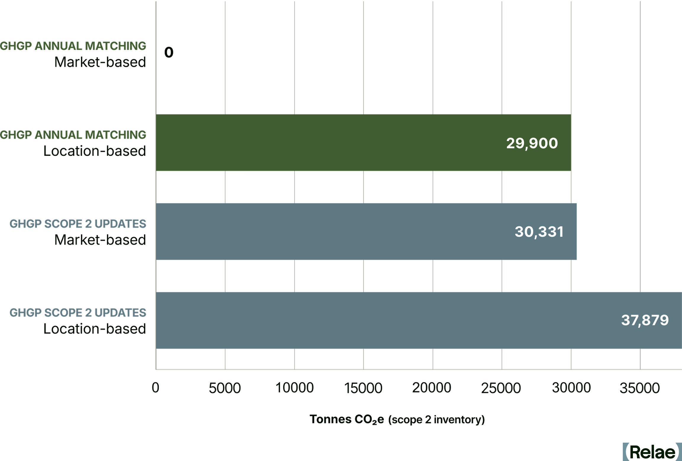
Understanding this emissions gap is the essential first step for buyers to make informed decisions about which instruments to retain, which contracts to renegotiate, and where new investment will matter most. If the proposed scope 2 revisions are enacted, companies procuring clean energy will be disincentivized from buying RECs sourced from variable renewables in distant locations, and instead will find it more favorable to invest in same-grid clean, firm generation, such as geothermal, nuclear, and renewables plus storage. RECs from these projects would qualify to be retired against market-based scope 2 emissions under the proposed revisions, where today's distant-wind or off-peak-solar RECs would not.

Where Pressure Is the Highest: ERCOT and PJM

Two markets stand out for projected hyperscaler load growth: PJM, which covers the extended mid-Atlantic region, and ERCOT in Texas. Both are on track to absorb massive increases in data center demand over the next decade, and both expose the limits of annual REC accounting in ways that will be hard to ignore under the new proposed framework.

PJM: 60% Fossil Generation Means High Marginal Emissions

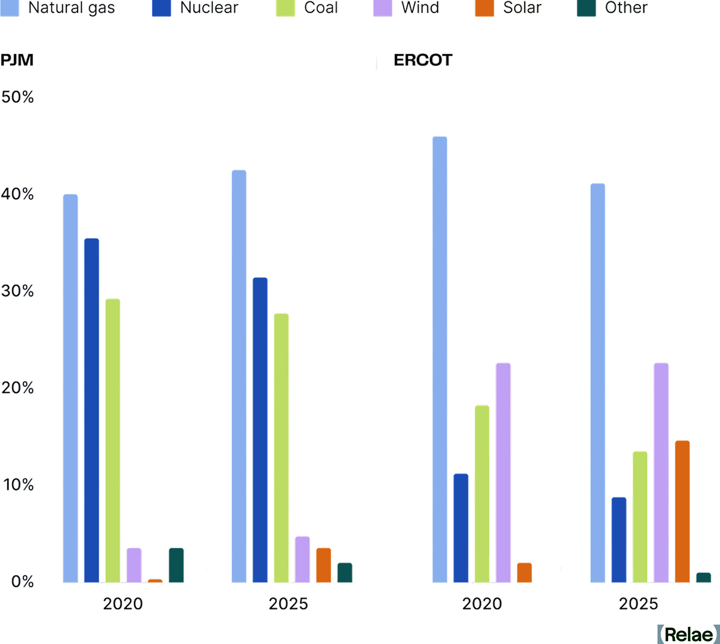
PJM is one of the largest and most complex wholesale electricity markets in the world. Its generation mix still includes 60% coal and natural gas, which means hourly emissions intensity remains high, particularly during evening peaks and grid stress events when fossil generation dominates the dispatch stack. 

Buyers relying solely on annual REC retirement may show low market-based scope 2 emissions today, but a 24/7 analysis tells a different story. For PJM-based buyers, this means hourly matching gaps will be largest during evening and overnight hours, when nuclear and storage become disproportionately valuable relative to additional solar.

ERCOT: Solar and Wind Don’t Peak When Demand Does

Texas has abundant wind and solar, with solar generation growing nearly 7x since 2020, but those resources don’t always run when demand peaks. While fossil-based generation has declined since 2020, it still comprises more than half of ERCOT’s generation. Solar dominates midday, wind peaks in the evening, and natural gas fills the gaps, especially during high-demand evenings or extreme weather events. 

Buyers with large ERCOT footprints may find that VPPA portfolios, which generate most of their clean energy in off-peak hours, already satisfy the proposed location-based test but fail on hourly matching. Battery storage and demand flexibility could help bridge the gap.

Figure 3 below quantifies that gap in both markets by showcasing the carbon-free energy (CFE) score in ERCOT and PJM, as well as the additional capacity required for a 4 GW load to achieve a 100% CFE target. The CFE score is the share of grid-supplied electricity in a given hour that comes from carbon-free sources, and is the metric the proposed scope 2 revisions would use to evaluate hourly matching. A 100% CFE target means electricity consumption is matched to carbon-free generation in every hour of the year.

In the left panel, a representation¹ of each market's 2030 hours are sorted by grid (CFE) score, from the dirtiest hour on the left to the cleanest on the right. Neither grid approaches 100% carbon-free on its own, and the shaded areas represent the unmatched hours a buyer claiming 100% clean energy through annual instruments would actually carry under 24/7 accounting. The gap is the maximum unmatched hours a buyer might be exposed to, as some RECs procured through annual matching may qualify under the new rules, if satisfying the locational and hourly requirements.

The right panel translates that gap into action. The additional co-located clean generation and storage required to serve a representative 4 GW load (roughly 5% of the forecast 2030 C&I load in ERCOT and 4% in PJM) at a 100% hourly CFE target, on top of what the underlying grid already provides.

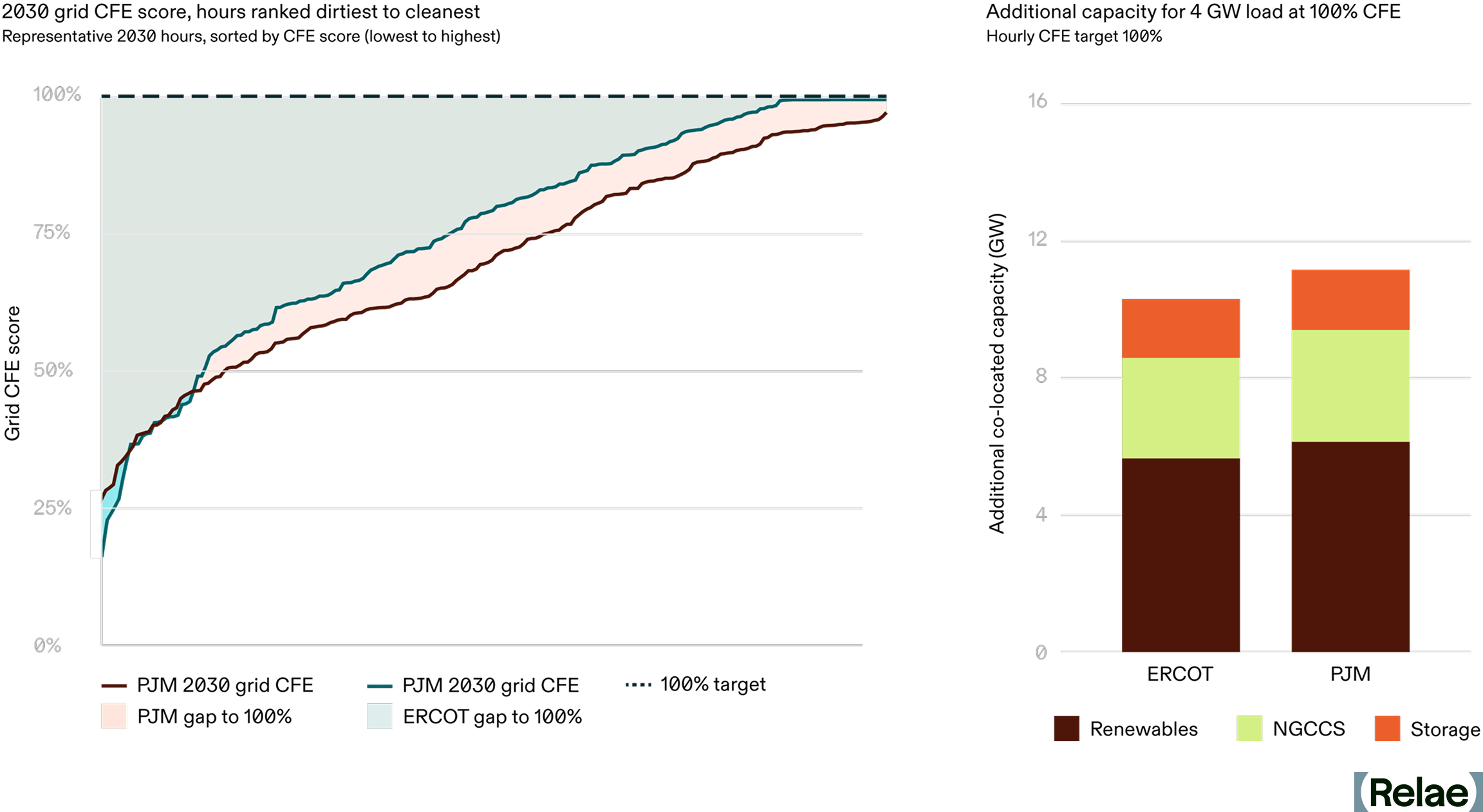
A few patterns are worth highlighting. First, the left panel confirms that PJM’s grid will still spend materially more hours below 100% carbon-free than ERCOT’s in 2030, a direct consequence of the coal- and gas-heavy generation mix described above. Notably, ERCOT's curve reaches 100% in a meaningful share of hours (windows when the grid is running entirely on carbon-free resources), while PJM's never does, meaning some fossil generation is dispatched in every hour.  

Second, the ISO a buyer operates in drives a meaningful difference in build-out: hitting 100% hourly CFE for a 4 GW load takes 9.6 GW of additional capacity in ERCOT and closer to 10.5 GW in PJM. This indicates the advantage of achieving hourly and locational matching in already clean grids, which may influence a buyer choosing where to site new workloads. 

Renewables have the largest share of the additional capacity in both markets (5-6 GW), paired with significant long-duration energy storage (~2 GW), while natural gas with CCS provides meaningful clean, firm capacity (~3 GW). ERCOT’s storage share of capacity is slightly larger, reflecting the midday-solar/evening-load mismatch, while PJM leans a bit more on natural gas with CCS, where clean, firm generation does more of the heavy lifting due to lower wind speeds and solar irradiance than Texas.

The right panel also illustrates why clean, firm technologies (natural gas with CCS, advanced nuclear, and enhanced geothermal) are likely to be included alongside renewables and batteries in any serious 24/7 portfolio. With only renewables and batteries, hitting the same target requires about double the total generation and storage capacity. In both markets, targets that look achievable today on an annual REC basis will require materially more capital and a different mix of resources, under 24/7 accounting. 

Top Questions Large Power Buyers Need to Model Before the Rules Change

The GHG Protocol revisions are not finalized, and the timing of any mandate remains uncertain, which is exactly why modeling cannot wait.

A useful self-test for any large power buyer is: can your team answer the following today with defensible numbers?

• What is your hourly CFE score across your largest load centers, and how far does it sit from your reported market-based emissions?
• Which of your existing VPPAs and REC contracts hold value under 24/7 accounting, and which become effectively stranded?
• What mix of resources delivers the incremental clean, firm capacity that closes your gap in PJM, ERCOT, or wherever your load is concentrated at the lowest cost?
• If your next gigawatt of load were sited in a different ISO, how would your emissions position change?

Clean firm projects do not appear off the shelf. Advanced nuclear, enhanced geothermal, and natural gas with CCS all carry multi-year development timelines, and corporate offtake agreements are often what get these projects financed in the first place. Buyers who engage now help shape the project pipeline that will be available in their target markets in 2030, and can lock in offtake terms before competition for the most valuable sites tightens. Buyers who wait until the methodology is final will be working with shorter lead times, fewer development partners, and less leverage to specify projects that fit their load profiles and hourly matching needs.

Frequently Asked Questions

What is 24/7 hourly matching, and how does it differ from today's REC accounting?

Today's scope 2 accounting lets companies retire renewable energy certificates (RECs) from any grid, at any time of year, to offset their emissions. The GHG Protocol's proposed 24/7 hourly matching would require RECs to come from clean generation on the same grid, in the same hour a facility consumes power, making most of today's location-agnostic RECs ineligible for market-based accounting.

Why are PJM and ERCOT under the most pressure from this shift?

Both markets are absorbing the fastest-growing data center load in the country, and both still lean on fossil generation to meet demand outside peak renewable hours. PJM's generation mix is 60% coal and gas, while ERCOT's solar and wind often don't peak when demand does, so buyers in these markets face the largest gaps between their annual REC claims and their actual hourly carbon-free energy score.

How much additional clean capacity does it take to close the gap?

Relae's modeling finds that serving a 4 GW data center load at 100% hourly carbon-free energy requires 9.6 GW of additional clean capacity in ERCOT and 10.5 GW in PJM. That capacity mix leans on renewables and long-duration storage in both markets, with natural gas with CCS playing a larger role in PJM, where wind and solar resources are weaker.

What should power buyers do before the GHG Protocol revisions are finalized?

Start modeling now. Buyers should know their hourly carbon-free energy score, understand which existing VPPAs and REC contracts hold value under 24/7 accounting, and identify the lowest-cost mix of clean, firm resources that closes their gap. Clean firm projects like advanced nuclear, enhanced geothermal, and natural gas with CCS take years to develop, so buyers who engage early have more influence over the project pipeline and better offtake terms.

Modeling the 24/7 Emissions Gap with Relae

For large power buyers assessing what the proposed GHG Protocol revisions mean for their power procurement portfolio, Relae's Advanced Power Emissions Analysis solution models the gap between current market-based reporting and what 24/7 accounting would reveal—by market, load profile, and technology stack. 

Key Takeaways

• Accurate load forecasting is needed to distinguish and prioritize real demand, align capital deployment, and reduce delays in bringing new power capacity online. Traditional load forecasting was built for predictable, gradual demand growth, not for the scale, uncertainty, and dynamic behavior of data centers. 
• The system-level fix to data-center load forecasting requires probabilistic, more frequent, category-specific methods paired with mandatory data standards and policy alignment. Together, these give planners visibility into the range of possible futures and the likelihood of each. 
• Without that fix, today's forecasts conflate real demand with speculative submissions, reducing accuracy. Inaccurate forecasting in either direction is expensive: underbuild adds friction to economic development; overbuild risks raising retail rates. Both can erode public trust in planning.
• Behind-the-meter generation (BTM) and load flexibility can help achieve speed-to-power in the near term. Just 1% data-center flexibility could unlock 100 GW—more than the entire US nuclear fleet.

Load Growth Is Increasing, Uncertain, and Concentrated

For two decades, US electricity demand was flat. Utilities, transmission planners, and corporate buyers built their planning models around that reality. Then AI workloads changed it.

AI load growth is large, uncertain, and concentrated in major power markets. While load forecasting projections vary across studies, the trajectory is clear: electricity demand is scaling faster than the bulk power grid was designed to handle. Accurate load forecasting is needed to distinguish and prioritize real demand, align capital deployment, and reduce delays in bringing new power capacity online.

On April 30, 2026, Relae (formerly Carbon Direct) hosted a Trellis Group panel on load forecasting in the AI era. Panelists included Derya Eryilmaz, PhD, Vice President of Power Commercialization at Relae; John Miller, Director of Transmission Policy at the Corporate Energy Buyers Association (CEBA); Daniel Padilla, Strategy and Business Development Lead at Emerald AI; and Sam Hodas, Head of US Government Affairs at National Grid. Jake Mitchell, Director of Climate Tech Innovation at Trellis Group, moderated.

The conversation explored where load forecasts fail, what they cost, how to fix them, and near-term solutions to overcome grid constraints. Here is what the panel found.

What Is Load Forecasting?

Load forecasting is the practice of predicting how much electricity will be consumed across a region, at what times, and under what conditions. It informs the major capital and procurement decisions on the grid: where to build transmission, how much generation to procure, what capacity to bid into wholesale markets, and how corporate buyers secure clean, firm power.

Long-term forecasts inform multi-year decisions about transmission and generation. Short-term operational forecasts inform real-time grid operations and trading. The two often sit in separate workflows, but short-term operational forecasts should feed into long-term system planning to improve accuracy as demand patterns shift.

The Bulk Power Grid Is Under Strain

Large power users face constraints on clean, firm power, transmission capacity, multi-year interconnection queues, and aging infrastructure. The strain is most acute in PJM Interconnection (PJM) and the Electric Reliability Council of Texas (ERCOT), the two US markets expected to see the most significant load growth. Each constraint raises the cost of getting load forecasts wrong.

Hodas from National Grid describes the operational reality on the utility side: aging infrastructure inherited from a different demand era. “We’ve got transmission lines that are 70 to 100 years old in New York and Massachusetts, some of the oldest in the country, still in operation.” Replacing or upgrading that infrastructure requires investment, and ratepayers are already pressed. 

Why Today’s Load Forecasts Fail

Traditional load forecasting was built for predictable, gradual demand growth, not for the scale, uncertainty, and dynamic behavior of data centers. 

Most utilities and Independent System Operators (ISOs) produce load forecasts on annual or biannual cycles. They aggregate submissions from individual customers, run that data through a deterministic single-peak load estimate against a single capacity scenario, and pass the consolidated forecast up to regional planners. Regional Transmission Organizations (RTOs) roll those bottom-up utility forecasts into a regional view. 

This worked when demand was flat and predictable. It no longer works with nonlinear growth driven by data centers. Eryilmaz from Relae identifies key structural limitations. 

Four Structural Limitations to Traditional Forecasting Methods

• Over-stating and double-counting. Data centers bid into multiple regions while shopping for power, inflating regional forecasts and blurring the line between real and hypothetical demand—the speculative-load problem.
• Deterministic models (vs probabilistic models). Most planning runs a single peak load estimate against a single capacity scenario, missing the geographic concentration and uncertainty inherent in integrating large loads into the system.
• Aggregated submissions. Utilities report large loads as a single block of gigawatts, with no resolution into workload type, ramp schedule, or operational shape. Planners reverse-engineer peak-demand assumptions rather than measure them.
• Infrequent cadence. Annual or biannual forecasts cannot catch an 80% queue reduction or a multi-gigawatt addition between cycles.

The Speculative-Load Problem

The core challenge in load forecasting is distinguishing real versus hypothetical load. While data center electricity demand is projected to grow by 13-27% annually through 2028, the majority of the projects in the data center queue may not materialize, inflating regional load forecasts.

American Electric Power's Ohio utility (AEP Ohio) introduced a tariff requiring data centers to put up firm financial commitments before getting in line for grid connection. Its interconnection queue dropped from 30 gigawatts to 5.6 gigawatts. More than 80% of the submitted load was speculative: projects that disappeared once commitment became required.

ERCOT shows the same overstatement problem on a larger scale. Roughly 225 gigawatts of data center demand sits in the ERCOT queue against a historic system peak of 85 gigawatts. Texas Senate Bill 6 introduced similar financial obligations for new loads, but those rules apply only to interconnections after 2025, and the cleanup of speculative demand has not yet materialized.

The speculative-load problem shows up in interconnection times. An average new project in PJM can wait 4 to 5 years to become operational. Some of that delay is a real backlog. The rest comes from the inability to distinguish real submissions from speculative ones.

As Eryilmaz puts it, “Load forecasting is actually the center of all of these problems. It is a tool to help planners make the right investment decisions.”

The Cost of Inaccurate Forecasting

As Miller from CEBA notes, “A single misforecasted project can swing a transmission plan by hundreds of megawatts.” Significant inaccuracies can erode public trust in the planning process in two main ways. Underbuilding adds friction to economic development and can limit corporate access to clean power markets. Conversely, overbuilding risks raising retail rates if capacity remains underutilized. 

The goal is to achieve right-sized infrastructure investment. When planning aligns with actual large load growth, it can be net beneficial to retail rates. By spreading fixed costs across more usage, significant new demand can put downward pressure on the rates via the “denominator effect.” 

On the other hand, forecasting variability can distort capacity procurement and interconnection queue prioritization. When load forecasts spike upward, grid operators like PJM have to scramble to buy additional electricity capacity on short notice. These emergency procurements lock in major dollar commitments on the basis of unstable forecast numbers. 

PJM, Midcontinent Independent System Operator (MISO), and Southwest Power Pool (SPP) have also reshaped their interconnection queues to make room for new large loads, but those queue priorities depend on the same forecasts that are unreliable in the first place. 

“There is no substitute for good backbone regional transmission planning,” Miller says. “Full stop. That is the enabler of all of the load growth that we’re talking about.”

BTM Generation and Load Flexibility: A Near-Term Bridge

Hyperscalers’ need for power is way faster than that of utilities and RTOs. Generation alone cannot scale fast enough to meet this new demand, and hyperscalers need speed-to-power.

As Eryilmaz frames it, behind-the-meter generation and load flexibility are interim solutions to the timing mismatch between data center urgency and the grid's slower build cycles. BTM generation and flexibility work differently:

• BTM is power generated on the data center's side of the utility meter, bypassing grid interconnection entirely. The structure gives operators large, reliable blocks of power without waiting years for grid approval.
• Load flexibility is the demand-side approach. A data center modifies its grid draw in response to grid signals. In practice, that can mean curtailing compute workloads during stress events, pre-cooling facilities ahead of a heat wave, drawing from on-site batteries or generators, or shifting workloads to data centers in less-constrained regions.

The Value of Load Flexibility

Relae’s power system modeling quantifies the dollar value of load flexibility in ERCOT. Load flexibility can eliminate forced load shedding risk, even at 40 gigawatts of data center buildout, preventing $5.5 billion in annual consumer welfare losses by curtailing an average of 5% of demand for under 1% of operating hours.

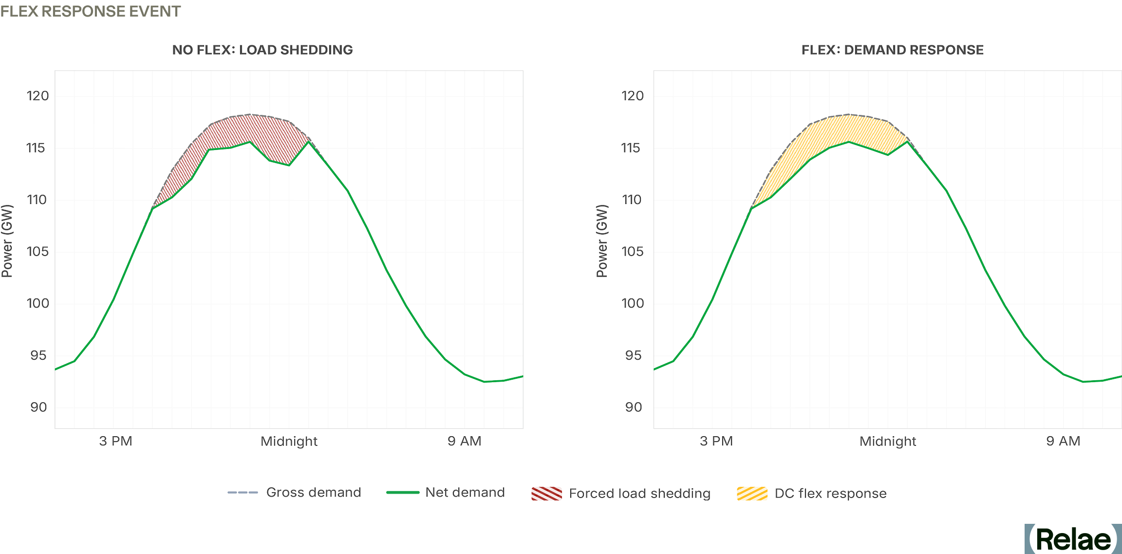
Padilla from Emerald AI reinforces the scale and value of load flexibility: “With just 1% flexibility, we can unlock 100 gigawatts of data centers across the US. That’s more than the entire US nuclear fleet.”

Silicon Valley Power, a municipal utility, is the first US utility to tie flexibility to interconnection speed: flexible data centers get connected faster. NVIDIA, EPRI, Digital Realty, and PJM are partnering on the Aurora AI Factory, the first purpose-built reference design for flexible AI data centers. 

But standardized policy for load flexibility is lagging. Padilla highlights this challenge: “Today, if a data center wants to be flexible, they have nowhere to point. We need standardized tariffs, interconnection rules, and product definitions for large loads that reward them with upsizing interconnection in response to flexibility.” 

Flexibility Takes Many Forms, but it Isn't Universal

Flexibility means accepting brief, predictable downtime, and some workloads can't tolerate it. Hospital systems and mission-critical enterprise applications need 99.999% uptime, the "five nines" standard. As Padilla puts it: "99.9% uptime, with brief and predictable curtailments, is plenty" for most AI workloads. That distinction determines which data centers can participate in flexibility programs.

Miller points out that compute-level flexibility is not always feasible. BTM batteries and virtual power plants (VPPs) are among the alternatives that can offset what data centers withdraw when the grid is stressed, even at facilities whose compute workloads cannot pause directly.

Better Load Forecasting: The Longer-Term Fix

While BTM generation and load flexibility can help address near-term speed-to-power, the longer-term fix is improving load forecasting methods and the standardization of data provided by the data centers themselves.

Eryilmaz outlines three technical shifts for better load forecasting:

• Embed short-term operational forecasting into long-term planning. Short-term spikes, weather risk, and reserve considerations carry direct implications for multi-year capital decisions. The line between operations and planning breaks down when growth is nonlinear.
• Replace deterministic models with probabilistic methods. Risk metrics like loss of load hours (expected hours per year that demand exceeds supply) and expected unserved energy (total expected energy shortfall) measure both how much capacity the system has and the conditions under which it might fall short. The North American Electric Reliability Corporation (NERC) has suggested both metrics as part of its reliability framework.
• Forecast load by category. Treating all data center load as a single block hides the differences in load profiles, operational schedules, and ramp-up timing that drive system planning.

Policy Alignment

Technical forecasting improvements only scale with policy alignment, and Miller proposes a two-part fix:

On the top-down side, RTOs need authority to take an independent view of utility-submitted forecasts. They should require milestones, such as firm financial commitments and secured financing, before counting a submitted load against the regional forecast. 

On the bottom-up side, state regulators set the rules that govern how individual utilities prepare their forecasts. Large load tariffs play a big role in how utility-level forecasts come together. Federal and state authorities need to row in the same direction. Hodas frames the same alignment from the utility side: “Grid investment unlocks economic growth, but for us to make those investments, we need regulatory certainty.”

Standardizing Large-Load Data

The Federal Energy Regulatory Commission (FERC) has since moved: in June 2026 it issued show cause orders directing six RTOs and ISOs—CAISO, ISO-NE, MISO, NYISO, PJM, and SPP—to revise or justify their large-load interconnection rules, and in July 2026 it directed NERC to develop computational-load reliability standards and registration criteria by the end of the year. Both are useful first steps. But as Eryilmaz argues, voluntary disclosure has not closed the gap.

The industry cannot meaningfully compare ISO forecasts when each utility submits load data in different shapes (e.g., using different methods and data standards) on different schedules. Mandatory submission requirements and published methodologies, applied consistently across utilities, ISOs, and state regulators, are the only path to forecasts whose components are actually comparable.

Getting Load Forecasting Right Starts Now

The system-level fix to improving forecasting is through probabilistic, category-specific methods paired with data standardization and policy support. Together, these account for the scale, uncertainty, and dynamic behavior of data center loads, and give planners visibility into the range of possible futures and the likelihood of each.  

All forecasts will be wrong to some degree, but as Miller puts it, “It's ultimately not about having a perfect prediction. It's about baking in methods to account for uncertainty.” These system-level improvements won't eliminate errors entirely, but they will minimize them, leading to more confident investment decisions and a grid better prepared for what's ahead.

Frequently Asked Questions

What is load forecasting, and why is it harder now with AI data center loads?

Load forecasting predicts how much electricity a region will consume, when, and under what conditions—the basis for where to build transmission, how much generation to procure, and how corporate buyers secure clean, firm power. It was designed for two decades of flat, gradual demand growth. Data center load is none of those things: it is large, geographically concentrated, arrives in gigawatt blocks with no disclosed operating shape, and can be withdrawn as quickly as it appeared.

What is speculative load in an interconnection queue, and how do planners tell it apart from real demand?

Speculative load is capacity requested by projects that may never be built — often the same data center bidding into several regions at once while shopping for power, which counts the same gigawatts more than once. The tested filter is a financial commitment: when AEP Ohio required firm commitments before queue entry, the utility's reported data center pipeline fell from about 30 GW to roughly 5.7 GW. Milestone requirements, independent RTO review of utility submissions, and mandatory data standards are the tools planners have.

Is load flexibility proven and scalable today, or still emerging?

The modeling case for load flexibility is strong; the commercial case is still early. Duke's Nicholas Institute found the 22 largest US balancing authority areas could absorb roughly 76–126 GW of new load if it accepts modest curtailment, and Relae's ERCOT modeling shows demand response eliminating forced load shedding risk at 40 GW of data center buildout, avoiding $5.5 billion in annual consumer welfare losses. What is still missing is the market plumbing—standardized tariffs, interconnection rules, and product definitions—so a data center willing to be flexible has somewhere to sign up.

What should a company look for when evaluating a region's load forecast?

Ask whether the forecast is probabilistic or a single deterministic peak, how often it is refreshed, and whether large loads are broken out by category and operating shape rather than reported as one block of gigawatts. Then ask what milestone or financial commitment a project must clear before its megawatts count toward the forecast. A forecast that cannot answer those three questions cannot tell you how much of the queue ahead of you is real.

[cta]

Key Takeaways

• On April 16, 2026, two weeks before the Department of Energy’s (DOE) April 30 deadline for action on the Large Load Proceeding, FERC, the Federal Energy Regulatory Commission, provided a significant update: 
  
  • FERC issued its compliance order on PJM's Bring Your Own Generation (BYOG) tariff; the order approved four interconnection paths, rejected two PJM proposals, and directed PJM to refile by May 18. 
  • FERC's June 2026 order settled a key question around enforcement mechanisms for co-located projects. FERC rejected PJM's Two-Strike proposal (which would have terminated contracts on second violation), allowing only penalties and suspension from the three new transmission services, materially reducing developer downside risk.
  • Notably, BYOG arrangements built on the rejected elements of the compliance filing face restructuring risk before that refile. For deals that clear it, however, energization could begin as early as this summer.
• These proceedings reflect the underlying industry concerns about speed, reliability, and cost equity, shifting the risks and costs of new generation from ratepayers to the large loads, such as data centers, themselves. 
  ‍
• Developers, investors, and project teams can use quantitative grid and load modeling to navigate these risks successfully, converting regulatory exposure into priced engineering decisions.

A New Rulebook for Bring Your Own Generation in PJM

PJM Interconnection (PJM) hosts the highest concentration of data center load growth in the US, managing regional transmission across 13 states in the Eastern US, and commercial operation dates for new generation projects in its current interconnection queue stretch into the early 2030s. Bring Your Own Generation (BYOG) has become the fastest speed-to-power path around that bottleneck. 

BYOG allows large loads, such as data centers, to draw power directly from a co-located generation source connected to the bulk power grid, enabling developers to avoid lengthy interconnection queues and costly transmission upgrades, while drawing limited to no power from the bulk power grid.

The Federal Energy Regulatory Commission’s (FERC) April 16 order is now the rulebook that governs the tariffs that facilitate these BYOG arrangements. Any deal built on the paths FERC closed off must now find a way to align with one of the four approved mechanics before PJM's May 18 compliance refile. Deals that clear the refile could begin to energize as early as this summer.

Below are the top questions the Relae power advisory team is fielding most from hyperscalers, large commercial power buyers, and power producers navigating the mechanics of PJM’s BYOG tariff and the engineering realities of running a co-located project. 

What Is Co-Location?

Co-location refers to a power generation facility sited in close proximity to a large load, such as a data center, that interconnects directly to the bulk power grid. The generator serves that load contractually via a power purchase agreement (PPA), with power flowing through the meter.

BYOG is the predominant co-location model in PJM. Under a typical BYOG arrangement, on-site generation covers the majority of the data center's load (~90%), with only a small residual portion (~10%) supplied from the grid. Each co-located project effectively functions as its own mini-grid, with explicit operational obligations that are less forgiving than standard transmission service (NITS).

Why Did FERC Keep Behind-the-Meter (BTM) and Co-Location Separate?

While BTM and co-location may look similar, they sit in different regulatory buckets. That said, the line between them is less clear-cut than it once was. FERC found existing BTM rules inadequate to address the grid impacts of large co-located loads and directed PJM to treat co-location as a distinct framework. 

At the same time, BTM rules, including how tariffs and distribution charges are applied, remain under revision in a separate PJM proceeding. The two tracks moving in parallel have contributed to the conflation of the frameworks in industry discussion.

How Does Co-Location Differ from BTM Generation?

• Co-location, as this order defines it, is a bulk grid-interconnected arrangement. The host generator remains on the same interstate grid, maintains its interconnection service agreement, and continues exporting power to the grid. The co-located load connects through an approved interconnection mechanic and takes transmission service under a PJM tariff product.
• BTM is a distinct arrangement. The generator sits on the consumer's side of the utility meter and serves the load through a private line, without an interconnection agreement. The load may typically have a grid connection; however, in some circumstances, the generation may be fully off-grid or islanded. By setting a megawatt (MW) threshold for BTM, larger loads with co-located generation may no longer net out their load to reduce transmission and grid charges. FERC's jurisdiction over a BTM arrangement is narrower, and the tariff mechanics that apply to co-location do not apply in the same way.

FERC's rejection of PJM's proposed BTM rule changes illustrates this distinction. The commission is keeping the two categories separate on purpose. Ultimately, FERC’s intention seems to signal that large loads co-located with generation may not be adequately reflected in grid and transmission upgrade costs when these assets are behind the meter. Historically, BTM assets were exempt from these costs because their relatively insignificant power contributions had no meaningful financial impact on the bulk power grid.

That said, the BTM track is still moving. PJM's BTM application rules, including the netting-off mechanism that lets BTM loads avoid utility tariffs, remain under review in parallel proceedings.

For developers, regulatory clarity on co-location and BTM is increasingly critical. In April 2025, FERC upheld its rejection of the Talen-Amazon Susquehanna nuclear BTM interconnection agreement proposal, declining to rehear arguments on the initial decision. To many experts, the split ruling signaled that the structure of PJM’s interconnection service agreement (ISA) is inadequate for large loads operating behind the meter. 

However, in the initial challenge to the Talen-Amazon proposal, utility companies argued that the arrangement would unjustifiably shift transmission costs to other PJM customers. Ultimately, in June 2025, Talen Energy entered into a 1,920 MW, front-of-the-meter power purchase agreement with Amazon Web Services, which does not require FERC’s approval. 

FERC Has Always Regulated Generators, Not Loads. What Changed?

The April 16 order lands inside a larger jurisdictional shift. FERC does not typically regulate load interconnection; its authority sits with the bulk power grid. Under Orders 888 and 2003, FERC has regulated how generators connect to that system (with standardized study deposits, readiness requirements, and withdrawal penalties) while load interconnection has historically been regulated at the distribution level under state jurisdiction.

That generation-only approach to FERC regulation worked for three decades. Now, the scale of AI data centers and other large loads creates interstate impacts that state-level load regulation cannot fully address. Generation co-location breaks the pattern by routing the load through a FERC-regulated generator interconnection agreement rather than a state-regulated load-serving entity, pulling it into federal jurisdiction.

In December 2025, FERC declared PJM's existing interconnection rules (tariff) unjust and unreasonable in the PJM Co-Location Order and directed PJM to revise the tariff. The April 16 order is FERC's review of that rewrite. 

As FERC Commissioner David Rosner wrote in his concurrence to the December 2025 PJM Co-Location Order: "We are trying to meet surging demand while upholding two fundamental values that underpin the electric industry in our country: first, that all customers have a right to receive electric service on a timely basis, and second, that electric service should be reliable and affordable for all customers. Given the scale of new large loads putting demand on our grid today, it is clear that fostering both of these values requires intervention."

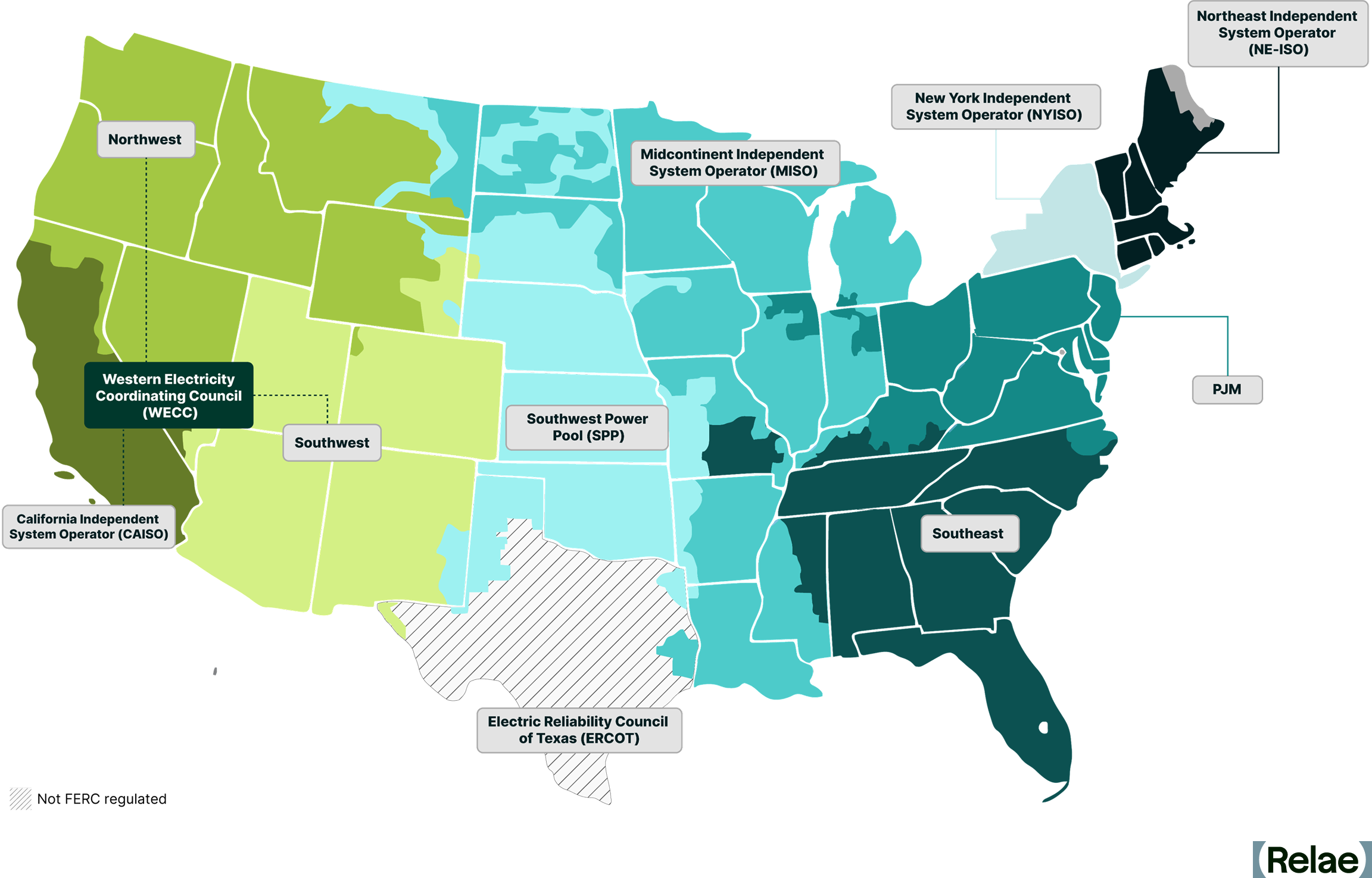
Which Four Interconnection Mechanics Did FERC Approve?

The April 16 order (Docket ER26-1088-000, 195 FERC ¶ 61,030) approves four ways for a data center to plug into the PJM grid. Each solves a different bottleneck: available capacity, queue position, study timing, or pre-studied capacity. All four rely on existing PJM and FERC tariff mechanics rather than new constructs, a deliberate choice to reduce legal exposure and speed up adoption. 

1. Sub-full-capacity interconnection service (available capacity). The data center co-locates with an existing host generator, and interconnects at less than the host generator's full capacity, using the portion of the existing interconnection rights the generator does not need.
2. Request acceleration at Decision Points I and II (queue position). Co-located load applications can move ahead of the standard queue at defined checkpoints, subject to PJM's study results. Co-located loads place less demand on the bulk power grid than new large loads without co-located generation, justifying the accelerated treatment. To qualify, projects must demonstrate there will be no significant network updates required or network impact, among other readiness milestones. 
3. Provisional Interconnection Service, or PIS (study timing). Interim interconnection services are provided during the full study, giving developers a bridge to early operations.
4. Surplus Interconnection Service, or SIS (pre-studied capacity). Use of unused capacity at an already-studied generator’s interconnection point, without triggering a new full study.

The four mechanics are different ways of answering the same operational question—how a co-located data center plugs into the grid without triggering a multi-year re-study of the host generator's interconnection—enabling faster speed-to-power.

Which Generators Gain Most From Surplus Interconnection Service?

SIS is the most commercially interesting of the four mechanics for existing generator owners because it monetizes previously stranded capacity.

The generators that benefit most include:

• Retiring or derated thermal units with unused megawatts of interconnection rights at high-value points (for example, retiring coal plants in PJM's eastern and mid-Atlantic footprint).
• Existing nuclear and large thermal plants near concentrated load growth, particularly in Dominion, American Electric Power (AEP), and ComEd territory (the Northern Virginia, Columbus, and Chicago metro zones), where PJM load is most concentrated.
• Storage-paired assets where the underlying generator has capacity headroom that the storage does not fully use (for example, solar-plus-storage or gas-plus-storage sites where the battery sits below the full interconnection rights).

For illustration, a host generator running at roughly 85% of its interconnection rights with a forced outage rate near 5% has material surplus capacity (10%) available to a co-located load, depending on how PJM studies the combined profile.

Owners of underutilized interconnection rights now have an approved tariff path to extract value from them by attracting data centers to co-locate with these generators.

What Transmission Service Does a Co-Located Load Receive?

Connecting to the bulk power grid and taking service from it are two separate decisions. PJM's default transmission service for any load on the system is the Network Integration Transmission Service (NITS), the standard contract for firm power year-round. NITS commits PJM to serve a customer’s full load at any and all times, meaning that PJM may need to wait for generation and/or transmission upgrades before offering it to a large load. 

Recently, PJM reopened its generation interconnection queue after pausing to study its backlog of proposed projects. With 800 proposed projects representing approximately 220 GW in new capacity in 2026, this growth signals progress, but it does not address the underlying permitting and financing challenges that have prevented projects already in the queue from being built.  

The BYOG mechanics are variations that waive or defer parts of NITS for faster speed-to-power. PJM delivers the resulting service through three tariff product types:

1. Firm contract demand: The co-located load holds firm transmission service (consistent with most aspects of NITS) and operates like any other firm load on the system. Availability is site-specific, depending on the point of interconnection. Unlike other NITS customers, entities contracting firm contract demand transmission on behalf of co-located loads cannot exceed the contracted demand level, and loads would be subject to a penalty if they withdraw additional energy beyond the contracted demand capacity. 
2. Non-firm contract demand: The load accepts interruption risk in exchange for faster interconnection or lower-cost service, making it better suited to loads with operational flexibility. It is available at more interconnection points than firm service, but power delivery is subject to curtailment based on real-time grid conditions. This service intends to provide brief and intermittent energy access from the bulk power grid, during available periods, under unanticipated circumstances, such as downtime for the co-located generator. 
3. Interim NITS: A bridge product that provides firm service on an interim basis while the co-located generator is still under construction. The load energizes early; once the generator and any transmission upgrades are complete, the project transitions to a standard NITS arrangement, and the generator can participate in the broader PJM market. However, while the load pays the NITS rate, the load is subject to curtailment under system emergency conditions, posing reliability challenges. 

In practice, a 1,000 MW data center co-located with a 900 MW on-site generator would request 100 MW from PJM under one of these three products.

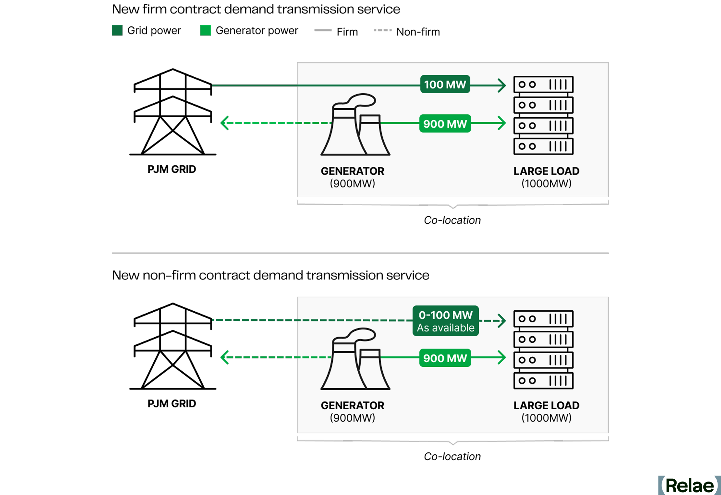
The interconnection mechanic (how the load connects) and the tariff product (what service the load receives) are two distinct decisions. For example, in the case of an interim NITS, a data center and co-located load could connect through a Provisional Interconnection Service (PIS). Other co-located loads may connect by submitting a request for acceleration at Decision Points I and II to secure firm contract demand service. The connection mechanism and tariff will vary based on each co-located load’s unique characteristics and project configuration. 

For clients evaluating specific sites, the right path depends on how much of the host generator's interconnection capacity is available, how sensitive the load is to interruption, and how fast the site needs to energize. Grid modeling allows project teams to quantitatively assess their risk exposure before committing to a tariff product. 

Which Two PJM Proposals Did FERC Reject?

Two elements of PJM's original filing did not make it through the April 16 order.

1. Point of Change in Ownership substitution: PJM proposed swapping in "Point of Change in Ownership" for FERC’s mandated term "Point of Interconnection" in the definition of Co-Located Load. FERC rejected the swap as an unexplained deviation from the Co-Location Order's definition and because it could let transmission owners delay or effectively veto the Point of Change in Ownership location, creating uncertainty for co-located projects.
2. BTM application-rule changes: PJM tried to fold changes to its BTM application rules into this same compliance package. FERC rejected that on the ground the changes did not fall within the scope of the initial order. BTM remains a separate regulatory track; the April 16 order does not settle it.

Project configurations built on either rejected proposal need restructuring before PJM's May 18 refile.

The order also directs PJM to add the PIS definition to the Open Access Transmission Tariff (OATT), Part I, section 1 (paragraph 26), and flags items in paragraph 29, including assessment of the reliability of co-located loads paired with electric storage, as out of scope. 

These determinations should not be seen as FERC rejecting these tariff changes, but rather deeming them outside the scope of the order. They are open questions that belong in a separate docket. The direction to include PIS while declining to address issues not included in the compliance proceeding demonstrates FERC’s focus on speed-to-power, clarifying the rules for new co-located generators to connect to the grid more quickly.  

What Is the Two-Strike Reliability Rule, and Why Does it Matter?

The rules for violating a co-location interconnection service agreement are still being developed, but FERC has urged PJM to issue robust protections to maintain reliability and cost allocation equity. 

For both firm and non-firm contract demand transmission service, PJM will apply a penalty rate to transmission service customers who withdraw more energy from the grid than was contracted. The precise design of these rates for unreserved use is scheduled for a paper hearing this spring; however, developers should cautiously size and appropriately model load and generation sizes, as the penalties for jeopardizing PJM’s reliability are not limited to rates. 

While penalty rate design for unreserved use is underway, PJM proposed a strict Two-Strike reliability rule for co-located projects. If a co-located customer failed to adequately implement automated loadshedding or generator tripping mechanisms during unusual grid conditions, PJM has previewed severe consequences:  

• First strike: a 120-day operational pause for review.
• Second strike: termination of the transmission service contract and return to the NITS interconnection waitlist.

The entire purpose of pursuing a co-located large load configuration is to ensure speed-to-power while maintaining reliability. In a June 2026 order, FERC conceded that there are legitimate reliability concerns with co-located generation misoperation; however, PJM’s proposal to disqualify customers with multiple misoperations is unnecessarily strict. FERC ultimately agreed PJM has the authority to charge penalties to and temporarily suspend services for customers that fail to shed load or curtail, but cannot disqualify customers for misoperation. Data centers will need to rigorously model and design their co-located load and generator facilities with the understanding that multiple reliability violations could strand billion-dollar assets for multiple years. 

Which BYOG Deals Need Restructuring Before the May 18 Refile?

Any deal built around the Point of Change in Ownership substitution or the BTM application-rule changes that FERC rejected needs restructuring. 

In addition, co-located projects that relied on one of the four approved mechanics, but used PJM tariff language from the original December filing, may also need re-papering against the language PJM submits in its forthcoming May 18 compliance filing. Until PJM files that package and FERC accepts it, the operative document is the April 16 order itself.

Counterparties should confirm that operational controls, curtailment rights, and dispute mechanisms in the contract align with the proposed Two-Strike regime and the approved mechanics the project uses.

What Does Grid Modeling Reveal for a Co-Located Project?

Non-firm service is the lowest-cost tariff product for the portion of load the co-located generator does not serve, but availability depends on real-time grid conditions. Grid modeling is how developers size that exposure before signing.

Take the same 1,000 MW data center paired with a 900 MW on-site generator, contracting 100 MW of non-firm service for the residual load. Grid modeling might show non-firm power dropping out in roughly 15% of hours during the summer peak.

If the on-site generator also carries a 5% forced outage rate, the developer faces a meaningful probability of a compound event: grid supply drops out at the same moment the on-site unit trips offline.

In that window, the data center has three options, none of them free: 

1. Curtail load. 
2. Shift the load to another site. 
3. Draw more from the grid than the contract allows, which triggers a Two-Strike violation.

Grid modeling converts that risk into decisions the developer can price. A developer can test whether adding 50 MW of battery storage, contracting 150 MW of firm service instead of 100 MW of non-firm, or adding a smaller backup generator delivers the best risk-adjusted return.

Key Takeaways

• On May 4, 2026, the North American Electric Reliability Corporation (NERC) issued a rare Level 3 “Essential Actions” Alert in response to repeated events in which 1,000+ megawatts (MW) of computation load dropped off the bulk power system in seconds, leading to major grid stability issues.
• The pattern has since escalated: on July 22, 2026, a transmission fault in Ashburn, Virginia took more than 3 GW of data center load offline in seconds—roughly 3% of PJM demand at the time.
• NERC also published Reliability Guidelines that push the same concerns into long-term planning, explicitly recommending resource adequacy models that capture firm vs. flexible load, behind-the-meter resources, and AI training operating windows.
• For transmission operators and balancing authorities, the releases compel new scrutiny of how computational loads affect stability and resource adequacy. For hyperscalers and other large loads, those assessments now sit on the critical path: if operators cannot show through advanced modeling that they can integrate the new loads, interconnection and buildout plans stall.
• Meeting the bar takes advanced grid modeling at multiple time and spatial scales, from sub-second stability through long-horizon capacity and resource adequacy, to evaluate the role of large load portfolios considering demand response, storage, and co-located generation.

Why Grid Frequency Matters for Large Loads

When we turn on the lights or charge our phones, it’s easy to forget that electricity travels through the power grid as alternating current. Sixty times a second—far faster than our eyes can see—the flow of electricity alternates back and forth along the wires making up both the transmission and distribution parts of the North American grid. 

Power generation equipment and most large industrial loads are designed to work with this 60 Hertz (Hz) alternating flow and must be synchronized precisely to this rhythm to function. Grid synchronization is so important that it can even have geopolitical implications.

For some electrical equipment, getting out of sync with the grid’s frequency can lead to malfunctions or even physical damage and destruction. That’s why grid-connected equipment is protected by circuits that automatically disconnect from the grid (“trip offline”) if the grid frequency begins to deviate by even one percent. For minor equipment, this is easily managed. However, when large amounts of generation or load trip offline quickly, it can lead to rapidly cascading grid blackouts affecting tens of millions of people with costs in the billions.

Grid operators pay extremely careful attention to factors that could cause grid frequency to deviate. The grid’s frequency stays near 60 Hz only when total power generation and consumption (load) are closely balanced. If load suddenly drops below generation, physical rotating generators like gas turbines can begin to speed up, making grid frequency rise. 

This becomes particularly dangerous when large grid-connected loads all trip offline simultaneously because of minor frequency deviations or other factors. If these loads are large enough, they can trigger a cascading sequence of rising frequency and further equipment and generator trips, potentially causing a complete “grid collapse” blackout. The North American grid may be getting closer to this scenario. 

What Triggered NERC’s Highest-Urgency Alert

Data center load drops are now a documented grid stability threat. On May 4, 2026, NERC issued a rare Level 3 “Essential Actions” Alert—its highest-urgency notification—in response to a pattern of customer-initiated load reductions in which 1,000+ MW of computational load (data centers) dropped off the bulk power system (tripped offline) in seconds. These were “customer-initiated” because protection circuits at data centers detected problems with grid-supplied power and automatically disconnected to protect their sensitive computing equipment from electrical damage. 

Paired with a new Reliability Guideline on emerging large loads, the alert highlights the urgent need to better understand the potential for these events to cause grid instability or even blackouts. Together, these two documents reset the bar for the detailed grid modeling and planning needed for any utility, independent system operator (ISO), or hyperscaler with material data-center growth in its footprint.

How the Alert Reshapes Grid Interconnection

For utilities and ISOs, the alert and guideline raise the standard of evidence required to connect computational loads safely to the grid. Modeling assessments now sit on the critical path for large load interconnection decisions, and the same studies will increasingly inform reserve margin, transmission, and dispatch program designs.

For hyperscalers and other large loads, the consequence is direct. Plans that assume firm service without supporting analysis will face longer queues and tougher interconnection conditions. Buildout timelines now depend on whether utilities and ISOs can show, through stability and resource adequacy modeling, that the system can absorb the load and respond safely to its disturbances.

For storage developers, particularly long-duration and fast-responding assets, these events elevate the reliability value of rapid response and load-shifting resources. The same grid modeling improvements that capture flexible load behavior also surface storage's full reliability contribution.

For flexibility platforms, the same modeling work that satisfies NERC's expectations unlocks faster, cheaper interconnection. Demand response, large-load shifting, and co-located dispatch coordination are now both technical and commercial enablers.

A Higher Bar for Power Analysis

These pressures point to a higher bar for power analysis at multiple time and spatial scales, for utilities and the large loads they serve.

At sub-second to second timescales, electromagnetic transient (EMT) models capture fast electrical switching and the uninterruptible power supply behavior that determines whether a data center stays connected during a disturbance (“rides through”). The alert asks for these models to be more detailed, validated against actual equipment, and shared between large loads, transmission owners, and planners.

At seconds-to-minutes, dynamic stability simulation covers system frequency response, voltage recovery, and oscillation behavior after disturbances. NERC now expects annual stability studies and explicit load drop contingencies in planning files.

At hours-to-years, capacity expansion and production cost modeling determine whether the system has enough resources, in the right places, with the right flexibility, to keep up with computational load growth. NERC’s May 2026 Large Loads Reliability Guideline is most explicit at this scale, calling for resource adequacy studies that represent firm and flexible load components, behind-the-meter resources, AI training operating windows, and probabilistic scenarios across many weather, load, and outage combinations on a network-aware footprint. 

Rising to the Challenge

Since the alert was issued, its expectations have begun hardening into rules. Registered entities were required to report to NERC on their progress against the seven Essential Actions by August 3, 2026, and on July 16, 2026, FERC directed NERC to go further: to develop mandatory reliability standards for computational loads and revise its registration criteria, with the first standards and Rules of Procedure changes due December 31, 2026 and a second-phase work plan due March 1, 2027. NERC's Large Loads Action Plan anticipates new "Computational Load Owner" and "Computational Load Operator" registered entity types alongside the first three computational load standards. 

The practical consequence is that the modeling described above is no longer only good planning practice: utilities, ISOs, hyperscalers, and other large loads should expect the data-sharing, study, and commissioning expectations in the alert to return as auditable requirements, and should build the capability before the compliance deadline rather than after it. 

Frequently Asked Questions

What is a NERC Level 3 Alert, and what does it require?

A Level 3 “Essential Actions” Alert is the most urgent of NERC's three alert levels, reserved for risks that need immediate, documented industry response. The May 4, 2026 alert directed registered entities to take seven essential actions on computational load—covering modeling, system studies, commissioning, protection, fault recording, and direct operational communication with large load operators. Written responses were due to NERC by August 3, 2026.

Why do data centers disconnect from the grid during minor disturbances?

Data centers run voltage- and frequency-sensitive computing equipment protected by automatic transfer systems that switch to on-site UPS or backup generation the moment grid power looks abnormal. Those protection settings trip faster, and at smaller deviations, than conventional industrial loads, so a fault lasting milliseconds can move a gigawatt of demand off the system in seconds. Because the shift is customer-initiated, grid operators get no warning and no time to rebalance.

How does the alert change interconnection for hyperscalers and other large loads?

Modeling assessments now sit on the critical path for large load interconnection. A plan that assumes firm service without stability and resource adequacy analysis behind it will face longer queues and tougher interconnection conditions, because the utility or ISO has to be able to show the system can absorb the load and respond safely to its disturbances. In practice, buildout timelines are now tied to someone else's study queue.

What modeling do utilities and large loads need to meet NERC's expectations?

Electromagnetic transient (EMT) models validated against actual equipment for sub-second ride-through behavior; dynamic stability simulation with explicit load-drop contingencies for seconds-to-minutes frequency and voltage response; and capacity expansion and probabilistic resource adequacy modeling that separates firm from flexible load, represents behind-the-meter resources, and reflects AI training operating windows. The paired Reliability Guideline is most explicit about the last of these.